A Semi-Implicit, Three-Dimensional Model for Estuarine ... - USGS

More documents

Recommendations

Info

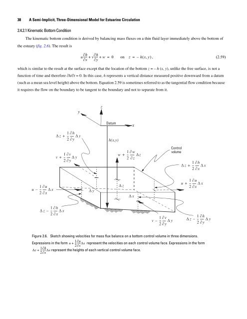
38 A Semi-Implicit, Three-Dimensional Model for Estuarine Circulation 2.4.2.1 Kinematic Bottom Condition The kinematic bottom condition is derived by balancing mass fluxes on a thin fluid layer immediately above the bottom of the estuary (fig. 2.6). The result is u ∂h ----- v ∂x ∂h + ----- + w = 0 on z = – h( x, y) , (2.59) ∂y which is similar to the result at the surface except that the location of the bottom z = – h (x, y), unlike the free surface, is not a function of time and therefore ∂h/∂t = 0. In this case, h represents a vertical distance measured positive downward from a datum (such as a mean sea level height) above the bottom. Equation 2.59 is sometimes referred to as the tangential flow condition because it requires the flow on the boundary to be tangent to the boundary and not to separate from it. 1 u -- 2 u ∂ – ----- Δ x ∂x 1 Δ z -- 2 h ∂ – ----- Δ x ∂x 1 Δ z -- 2 h ∂ + ----- Δ y ∂y 1 v -- 2 v ∂ + ---- Δ y ∂y y Δ y z Datum h(x,y) w Δ z x 1 -- 2 w ∂ + ------ Δz ∂z Δ x 1 v -- 2 v ∂ – ---- Δ y ∂y Control volume 1 Δ z -- 2 h ∂ + ----- Δ x ∂x 1 u -- 2 u ∂ + ----- Δ x ∂x 1 Δ z -- 2 h ∂ – ----- Δ y ∂y Figure 2.6. Sketch showing velocities for mass flux balance on a bottom control volume in three dimensions. 1 Expressions in the form u -- represent the velocities on each control volume face. Expressions in the form 2 represent the heights of each vertical control volume face. ∂u + -----Δx ∂x 1 Δz -- 2 ∂h + -----Δx ∂x
2.4.2.2 Dynamic Bottom Condition 2. Governing Equations and Boundary Conditions 39 The dynamic bottom condition is derived by applying the equation of motion to the thin fluid layer on the bottom (fig. 2.7). The equation of motion reduces to a balance between the stresses exerted by the boundary on the fluid and the stresses in the fluid exerted on the boundary. The stress vector exerted by the boundary is τ b and has components τ xb and τ yb acting along the boundary. The boundary slope in any direction is assumed sufficiently small so that the cosine of the vertical angle with the horizontal plane is unity. The balance of stresses results in and τ xb τ yb ∂h ∂h = – τ ----- – τ ----- + τ xx ∂x xy ∂y xz (2.60) τ ----- ∂h ∂h = – – τ ----- + τ (2.61) yx ∂x yy ∂y yz for the x- and y-directions, respectively. It is common practice to neglect entirely the slopes of the bottom boundary, ∂h/∂x and ∂h/∂y, so the first two terms on the right sides of the above equations can be eliminated. Then the dynamic equations become τ xb = τ and τ xz yb = τ , (2.62) yz which are the counterparts to equations 2.56 used at the surface. To evaluate equations 2.62, the fluid stresses (τ xz, τ yz) can be defined using equations 2.57 applied at the bottom of the estuary. It remains then to define the boundary stresses (τ xb, τ yb). τ xx τ yy 1 -- 2 τ ∂ xx – -------- Δ x ∂ x τ yx τ xy y 1 -- 2 τ ∂ yy + -------- Δ y ∂ y 1 -- 2 τ ∂ yx – -------- Δ x ∂ x 1 -- 2 τ ∂ xy + -------- Δy ∂ y z Datum h(x,y) τ xb τ yz τ xy x 1 -- 2 τ ∂ yz + -------- Δ z ∂ z τ yb 1 -- 2 τ ∂ xy – -------- Δ y ∂ y τ xz 1 -- 2 τ ∂ xz + -------- Δ z ∂ z τ yx τ yy 1 -- 2 τ ∂ yx + -------- Δ x ∂ x τ xx 1 -- 2 τ ∂ yy – -------- Δ y ∂ y Control volume 1 -- 2 τ ∂ xx + -------- Δ x ∂ x Figure 2.7. Viscous stresses on a bottom layer of a water body with boundary stress components τ xb and τ yb. Expressions in the form 1 τ -- represent the viscous stresses on each control volume face. yz 2 ∂τ yz + ---------- Δz ∂z
Page 1: In cooperation with the Interagency
Page 4 and 5: U.S. Department of the Interior Dir
Page 6 and 7: This page intentionally left blank.
Page 8 and 9: vi 4.2 Semi-Implicit One-Dimensiona
Page 10 and 11: viii Figure 5.6. Graph showing solu
Page 12 and 13: x Tables Table 2.1. Dimensionless n
Page 14 and 15: This page intentionally left blank.
Page 16 and 17: 2 A Semi-Implicit, Three-Dimensiona
Page 24 and 25: 10 A Semi-Implicit, Three-Dimension
Page 48 and 49: 2.4.1.2 Dynamic Surface Condition 2
Page 68 and 69: Water surface Water surface Level p
Page 70 and 71: h 1 h 2 h 3 h 4 h 5 h 6 z 1 ⁄ 2 z
Page 102 and 103:
88 A Semi-Implicit, Three-Dimension
Page 104 and 105:
Page 106 and 107:
Page 108 and 109:
Page 110 and 111:
Page 112 and 113:
Page 114 and 115:
100 A Semi-Implicit, Three-Dimensio
Page 116 and 117:
Page 118 and 119:
Page 120 and 121:
Page 122 and 123:
Page 124 and 125:
Page 126 and 127:
Page 128 and 129:
Page 130 and 131:
Page 132 and 133:
Page 134 and 135:
Page 136 and 137:
Page 138 and 139:
Page 140 and 141:
Page 142 and 143:
Page 144 and 145:
Page 146 and 147:
Page 148 and 149:
Page 150 and 151:
Page 152 and 153:
Page 154 and 155:
Page 156 and 157:
Page 158 and 159:
Page 160 and 161:
Page 162 and 163:
Page 164 and 165:
Page 166 and 167:
Page 168 and 169:
Page 170 and 171:
Page 172 and 173:
Page 174 and 175:
Page 176 and 177:
Page 178 and 179:
Page 180 and 181:
Page 182 and 183:
Page 184 and 185:
Page 186 and 187:
Page 188 and 189:
Page 190:
show all

A Semi-Implicit, Three-Dimensional Model for Estuarine ... - USGS

You also want an ePaper? Increase the reach of your titles

Delete template?

Save as template?