A Semi-Implicit, Three-Dimensional Model for Estuarine ... - USGS
A Semi-Implicit, Three-Dimensional Model for Estuarine ... - USGS
A Semi-Implicit, Three-Dimensional Model for Estuarine ... - USGS
You also want an ePaper? Increase the reach of your titles
YUMPU automatically turns print PDFs into web optimized ePapers that Google loves.
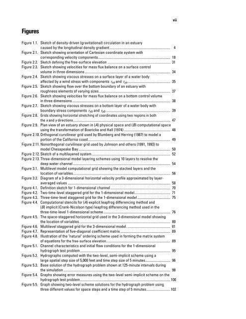
Figures<br />
Figure 1.1. Sketch of density-driven (gravitational) circulation in an estuary<br />
caused by the longitudinal density gradient.................................................................... 4<br />
Figure 2.1. Sketch showing orientation of Cartesian coordinate system with<br />
corresponding velocity components................................................................................. 18<br />
Figure 2.2. Sketch defining the free-surface elevation ............................................................... 31<br />
Figure 2.3. Sketch showing velocities <strong>for</strong> mass flux balance on a surface control<br />
volume in three dimensions................................................................................................ 34<br />
Figure 2.4. Sketch showing viscous stresses on a surface layer of a water body<br />
affected by a wind stress with components τxs and τys................................................ 35<br />
Figure 2.5. Sketch showing flow over the bottom boundary of an estuary with<br />
roughness elements of varying sizes................................................................................ 37<br />
Figure 2.6. Sketch showing velocities <strong>for</strong> mass flux balance on a bottom control volume<br />
in three dimensions.............................................................................................................. 38<br />
Figure 2.7. Sketch showing viscous stresses on a bottom layer of a water body with<br />
boundary stress components τxb and τyb ........................................................................ 39<br />
Figure 2.8. Grids showing horizontal stretching of coordinates using two regions in both<br />
the x and y directions............................................................................................................. 47<br />
Figure 2.9. Plan view of an estuary shown in (A) physical space and (B) computational space<br />
using the trans<strong>for</strong>mation of Boericke and Hall (1974) .................................................... 48<br />
Figure 2.10. Orthogonal curvilinear grid used by Blumberg and Herring (1987) to model a<br />
portion of the Cali<strong>for</strong>nia coast............................................................................................ 49<br />
Figure 2.11. Nonorthogonal curvilinear grid used by Johnson and others (1991, 1993) to<br />
model Chesapeake Bay....................................................................................................... 50<br />
Figure 2.12. Sketch of a multilayered system........................................................................................ 52<br />
Figure 2.13. <strong>Three</strong>-dimensional model layering schemes using 10 layers to resolve the<br />
deep water channel ............................................................................................................. 54<br />
Figure 3.1. Multilevel model computational grid showing the stacked layers and the<br />
location of variables............................................................................................................. 56<br />
Figure 3.2. Diagram of a 3-dimensional horizontal velocity profile approximated by layeraveraged<br />
values ................................................................................................................... 58<br />
Figure 4.1. Definition sketch <strong>for</strong> 1-dimensional channel ................................................................... 70<br />
Figure 4.2. Two-time-level staggered grid <strong>for</strong> the 1-dimensional model........................................ 71<br />
Figure 4.3. <strong>Three</strong>-time-level staggered grid <strong>for</strong> the 1-dimensional model ..................................... 75<br />
Figure 4.4. Computational stencils <strong>for</strong> (A) explicit leapfrog differencing method and<br />
(B) implicit (Crank-Nicolson type) leapfrog differencing method used in the<br />
three-time-level 1-dimensional scheme........................................................................... 76<br />
Figure 4.5. The space-staggered horizontal grid used in the 3-dimensional model showing<br />
the location of variables...................................................................................................... 80<br />
Figure 4.6. Multilevel staggered grid <strong>for</strong> the 3-dimensional model. ................................................ 81<br />
Figure 4.7. Representation of five-diagonal coefficient matrix ........................................................ 89<br />
Figure 4.8. Illustration of the "natural" ordering scheme used in <strong>for</strong>ming the matrix system<br />
of equations <strong>for</strong> the free-surface elevation........................................................................ 89<br />
Figure 5.1. Channel characteristics and initial flow conditions <strong>for</strong> the 1-dimensional<br />
hydrograph test problem..................................................................................................... 95<br />
Figure 5.2. Hydrographs computed with the two-level, semi-implicit scheme using a<br />
large spatial step size of 5,000 feet and time step size of 5 minutes............................ 96<br />
Figure 5.3. Base solution of the hydrograph problem shown at 125-minute intervals during<br />
the simulation........................................................................................................................ 98<br />
Figure 5.4. Graphs showing error measures using the two-level semi-implicit scheme on the<br />
hydrograph test problem.....................................................................................................100<br />
Figure 5.5. Graph showing two-level scheme solutions <strong>for</strong> the hydrograph problem using<br />
three different values <strong>for</strong> space steps and a time step of 5 minutes...........................102<br />
vii


