A Semi-Implicit, Three-Dimensional Model for Estuarine ... - USGS

More documents

Recommendations

Info

96 A Semi-Implicit, Three-Dimensional Model for Estuarine Circulation 5.2.1.1 Two-Level Scheme Figure 5.2 shows three computed hydrographs using the two-level, semi-implicit scheme described in section 4.2.1. Two of the solutions are based on computations using a coarse numerical grid size of Δx = 5,000 ft (1,524 m) and Δt = 5 minutes; the third solution is considered a “base solution” and is computed using an extremely small grid size that keeps the numerical error in the solution negligible. The base solution agrees to a high degree of accuracy with the solutions to this problem obtained using the other flow models tested by the USGS. All three solutions were computed with the number of iterations (niter) of the numerical scheme fixed throughout the simulation; the coarse grid solutions used values of niter = 1 and niter = 2, the base solution used niter = 5. Figure 5.2 indicates that a significant improvement in accuracy is gained by solving the coarse grid case using two iterations rather than one. The root mean square error (RMS e in table 5.1) of the solution measured against the base solution improved from 7.6 percent using niter = 1 to 2.7 percent using niter = 2. The improvement is due to a centering in time of the nonlinear coefficients of the finite-difference momentum equation by the iteration process, as discussed in section 4.2.1. Because the frictional attenuation of the routed hydrograph is significant, the backward-in-time evaluation of the frictional coefficient γ in equation 4.7 is mostly responsible for the large underestimation of the wave attenuation in the solution using niter = 1; also affecting the accuracy, but to a lesser degree, is the backward-in-time evaluation of the coefficient H in the pressure (water surface slope) and friction terms in equation 4.7. The centering in time of both γ and H by the iteration process raises the accuracy of the time integration scheme from first to second order. DISCHARGE, IN CUBIC FEET PER SECOND 800 700 600 500 400 300 200 Upstream Boundary 50,000 feet 100 0 100 200 300 400 500 TIME, IN MINUTES Δt = 5 seconds, Δ x = 50 feet, niter = 5 Δt = 5 minutes, Δ x = 5,000 feet, niter = 1 Δt = 5 minutes, Δ x = 5,000 feet, niter = 2 RMS error niter = 1 7.6 percent niter = 2 2.7 percent Figure 5.2. Hydrographs computed with the two-level, semi-implicit scheme using a large spatial step size of Δx = 5,000 feet (1,524 meters) and a time step size of Δt = 5 minutes. Solutions using one iteration (niter = 1) and two iterations (niter = 2) are compared against a base solution using a very small time and space step and five iterations (niter = 5). The hydrograph at the upstream boundary is also plotted. RMS, root mean square.
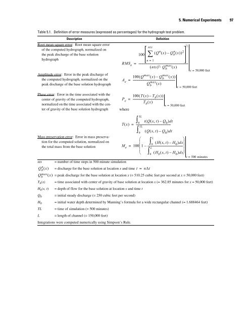
Table 5.1. Definition of error measures (expressed as percentages) for the hydrograph test problem. Description Definition Root mean square error: Root mean square error of the computed hydrograph, normalized on the peak discharge of the base solution hydrograph Amplitude error: Error in the peak discharge of the computed hydrograph, normalized on the peak discharge of the base solution hydrograph RMS e Phase error: Error in the time associated with the center of gravity of the computed hydrograph, normalized on the time associated with the cen- Pe = ter of gravity of the base solution hydrograph where A e 100 Q n nts n ( ( x) – Qb ( x) ) 2 ∑ n = 1 ( nts) 1 = ------------------------------------------------------------------------ ⁄ max 2 Qb ( x) 100 Q max max ( ( x) – Qb ( x) ) = ------------------------------------------------------------max Qb ( x) 100( T( x) – Tb( x) ) -------------------------------------------- Tb( x) x = 50,000 feet Tx ( ) = tQxt ( ( , ) – Q0)dt -------------------------------------------------- TL ∫0 ( Qxt ( , ) – Q0)dt Mass preservation error: Error in mass preservation for the computed solution, normalized on the total mass from the base solution Me = ⎛ L ⎞ ⎜ ∫0 ( Hxt ( , ) – H0)dx⎟ 100⎜1– --------------------------------------------------- ⎟ L ⎜ ⎟ ⎝ ∫0 ( Hb( x, t) – H0)dx⎠ t = 500 minutes nts = number of time steps in 500 minute simulation n Qb ( x) = discharge for the base solution at location x and time t = nΔt Qmax b ( x) = peak discharge for the base solution at location x (= 510.25 cubic feet per second at x = 50,000 feet) Tb(x) = time associated with center of gravity of base solution at location x (= 362.85 minutes for x = 50,000 feet) Hb(x, t) = depth of flow for the base solution at location x and time t Q0 = initial steady discharge (= 250 cubic feet per second) H0 = initial water depth determined by Manning’s formula for a wide rectangular channel (= 1.688464 feet) TL = time of simulation (= 500 minutes) L = length of channel (= 150,000 feet) Integrations were computed numerically using Simpson’s Rule. TL ∫0 5. Numerical Experiments 97 1⁄ 2 x = 50,000 feet x = 50,000 feet
Page 1:
In cooperation with the Interagency
Page 4 and 5:
U.S. Department of the Interior Dir
Page 6 and 7:
This page intentionally left blank.
Page 8 and 9:
vi 4.2 Semi-Implicit One-Dimensiona
Page 10 and 11:
viii Figure 5.6. Graph showing solu
Page 12 and 13:
x Tables Table 2.1. Dimensionless n
Page 14 and 15:
This page intentionally left blank.
Page 16 and 17:
2 A Semi-Implicit, Three-Dimensiona
Page 18 and 19:
Page 20 and 21:
Page 22 and 23:
Page 24 and 25:
10 A Semi-Implicit, Three-Dimension
Page 26 and 27:
Page 28 and 29:
Page 30 and 31:
Page 32 and 33:
Page 34 and 35:
Page 36 and 37:
Page 38 and 39:
Page 40 and 41:
Page 42 and 43:
Page 44 and 45:
Page 46 and 47:
Page 48 and 49:
2.4.1.2 Dynamic Surface Condition 2
Page 50 and 51:
Page 52 and 53:
Page 54 and 55:
Page 56 and 57:
Page 58 and 59:
Page 60 and 61: 46 A Semi-Implicit, Three-Dimension
Page 68 and 69: Water surface Water surface Level p
Page 70 and 71: h 1 h 2 h 3 h 4 h 5 h 6 z 1 ⁄ 2 z
Page 114 and 115: 100 A Semi-Implicit, Three-Dimensio
Page 160 and 161:
146 A Semi-Implicit, Three-Dimensio
Page 162 and 163:
Page 164 and 165:
Page 166 and 167:
Page 168 and 169:
Page 170 and 171:
Page 172 and 173:
Page 174 and 175:
Page 176 and 177:
Page 178 and 179:
Page 180 and 181:
Page 182 and 183:
Page 184 and 185:
Page 186 and 187:
Page 188 and 189:
Page 190:
show all

A Semi-Implicit, Three-Dimensional Model for Estuarine ... - USGS

You also want an ePaper? Increase the reach of your titles

Delete template?

Save as template?