A Semi-Implicit, Three-Dimensional Model for Estuarine ... - USGS

More documents

Recommendations

Info

82 A Semi-Implicit, Three-Dimensional Model for Estuarine Circulation 4.3.1.1 Momentum equations The solution of the momentum equations is separated into two stages in which first the explicit terms and then the implicit terms are evaluated. The separation is not a form of time-splitting but simply a grouping of terms for convenience in making the computer program modular and facilitating the presentation of equations. The finite-difference equation for the x-direction 1 momentum equation is written so it is centered within layer k at the horizontal point ( i + ⁄ 2)Δx , jΔy ; the explicit stage is represented by Ûi + 1⁄ 2, jk , = Ui 1⁄ 2 n – 1 + , j, k 2Δt ( ADVx) n ( CORx) n [ – + ( BCLINICx) n + – + ( HDIFFx) n 1 – ] i 1⁄ 2 + , j, k, (4.23) where the terms in brackets refer to the discretized form of the corresponding groupings of terms in equation 3.59. The bracketed terms are expanded fully using the leapfrog scheme and displayed in Appendix D (eqs. D.1–D.4). The symbol ˆ ( )in equation 4.23 denotes a solution for the layer volumetric transport which includes only the contribution from the explicit terms. The corresponding finite-difference equation for the explicit stage of the y-direction momentum equation is centered within layer k at 1 the point iΔx, ( j + ⁄ 2)Δy and is represented by n – 1 Ûi, j+ 1⁄ 2, k Uij , + 1⁄ 2, k 2Δt ( ADVy) n ( CORy) n ( BCLINICy) n – ( HDIFFy) n 1 – = + [ – – + ] i, j+ 1⁄ 2, k . (4.24) Here the bracketed terms refer to groupings of terms in equation 3.60, and they are expanded fully in Appendix D (eqs. D.5–D.8). All terms in equations 4.23 and 4.24, except horizontal diffusion (HDIFF), are centered in time at time level n to achieve secondorder numerical accuracy. The horizontal diffusion is written backward-in-time at time level n − 1 because the centering of that term can result in a weak instability; although formally this uncentered treatment of the horizontal diffusion introduces first-order truncation error, the actual size of the error should be miniscule. Presently in the model, the horizontal momentum exchange (or eddy viscosity) coefficient AH is defined at the center of each cell with whole integers of the indices i, j, k. The shear stress terms in equations 3.59 and 3.60 can be replaced by introducing the concept of the vertical momentum exchange (or eddy viscosity) coefficient: 34 τxz ∂u ------ = A ----ρ V , ∂z τyz ∂v ------ = A ---ρ V . (4.25) ∂z Then the finite-difference equation for the implicit stage of the x-momentum equation is written as n + 1 + , j, k= Ui 1⁄ 2 + ⎛ ⎝ n g n + 1 n + 1 n – 1 n – 1 ⎛( U⁄ h) i + 1⁄ 2, j, k– 1– ( U⁄ h) i + 1⁄ 2, j, k ui + 1 2 --------------------------------------------------------------------------- ⁄ , j, k– 1– ui + 1⁄ 2, j, k⎞ ⎜ + ------------------------------------------------------- ⎟ ⎝ n + 1 n – 1 ⎠ ⁄ , , – ⁄ ⁄ , , – ⁄ Δt – ----- hn i + 1⁄ 2, j, k Δx ρn ⎛ i + 1⁄ 2, j, 1⎞ ⎜--------------------- ⎟ ⋅ ( ζn + 1 ⎝ρn i + 1, j – ζn + 1 i, j + ζn – 1 i + 1, j – ζn – 1 i, j ) ⎠ i + 1⁄ 2, j, k Ûi + 1⁄ 2, j, k Δt⎜A Vi + 1⁄ 2 jk 1 ⋅ , , – ⁄ 2 hi + 1 2 j k 1 2 hi + 1 2 j k 1 2 n + 1 n + 1 n – 1 n – 1 n ⎛( U⁄ h) i + 1 2 A ⁄ , jk , – ( U⁄ h) i + 1⁄ 2, j, k+ 1 ui + 1 Vi ---------------------------------------------------------------------------- ⁄ 2, jk , – ui + 1⁄ 2, jk , + 1⎞⎞ – ⋅ + 1⁄ 2, jk , + 1 ⎜ + ------------------------------------------------------ ⎟⎟, (4.26) ⁄ 2 ⎝ n + 1 n – 1 ⎠⎠ ⁄ , , + ⁄ ⁄ , , + ⁄ hi + 1 2 jk 1 2 hi + 1 2 jk 1 2 34 The z-derivatives of u and v in equations 4.25 are mathematically undefined at the layer interfaces because the layer-averaged velocities are discontinuous there. A z-derivative at an interface is therefore understood to imply a finite-difference quotient involving the layer variables above and below the interface.
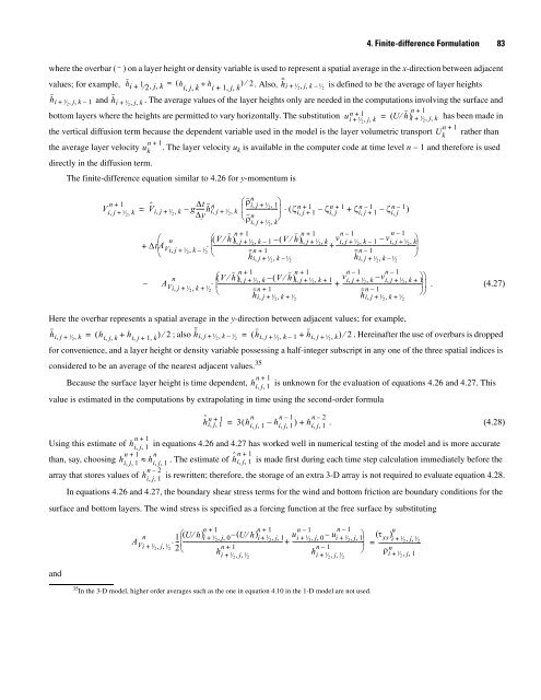
4. Finite-difference Formulation 83 where the overbar ( ) on a layer height or density variable is used to represent a spatial average in the x-direction between adjacent values; for example, hi + 1⁄ 2, j, k = ( h ijk , , + h ) ⁄ 2 i + 1, j, k . Also, hi + 1⁄ 2, jk , – 1⁄ is defined to be the average of layer heights 2 hi + 1⁄ 2, jk , – 1 and hi + 1⁄ 2, jk , . The average values of the layer heights only are needed in the computations involving the surface and bottom layers where the heights are permitted to vary horizontally. The substitution un + 1 n + 1 i + 1⁄ 2, j, k = ( U⁄ h) i + 1⁄ 2, j, k has been made in n + 1 the vertical diffusion term because the dependent variable used in the model is the layer volumetric transport Uk rather than n + 1 the average layer velocity uk . The layer velocity uk is available in the computer code at time level n − 1 and therefore is used directly in the diffusion term. The finite-difference equation similar to 4.26 for y-momentum is n + 1 , + , k = Vij 1⁄ 2 + , + , k g Δt ----- Δy V ˆ ij 1⁄ 2 – hn i, j+ 1⁄ 2, k ρi j 1 2 ρn i j 1⁄ 2 n ⎛ , + ⁄ , 1⎞ ⎜--------------------- ⎟ ⋅ ( ζn + 1 i, j+ 1 – ζn + 1 ij , + ζn – 1 i, j+ 1 – ζn – 1 ij , ) ⎝ ⎠ , + , k n + 1 n + 1 n – 1 n – 1 ⎛ , + , k⎞ ⎜ ------------------------------------------------------ ⎟ ⎝ ⎠ ⎛ n ( V ⁄ h) i, j+ 1⁄ 2, k – 1 – ( V ⁄ h) i, j+ 1⁄ 2, k Δt⎜A Vi ----------------------------------------------------------------------------- , j + 1⁄ 2, k – 1⁄ 2 n + 1 ⎝ hi, j+ 1⁄ 2, k – 1⁄ 2 vi, j+ 1⁄ 2, k – 1 – vi j 1⁄ 2 ⋅ + n – 1 hi, j+ 1⁄ 2, k – 1⁄ 2 n + 1 n + 1 n – 1 n – 1 n ⎛( V⁄ h) i, j+ 1⁄ 2, k – ( V⁄ h) i, j+ 1⁄ 2, k + 1 vi, j+ 1⁄ 2, k – vij , + 1⁄ 2, k + 1⎞⎞ – AVi ⋅ ----------------------------------------------------------------------------- , j+ 1⁄ 2, k + 1 ⎜ + ------------------------------------------------------ ⎟⎟. (4.27) ⁄ 2 ⎝ n + 1 n – 1 ⎠⎠ , ⁄ , + ⁄ , ⁄ , + ⁄ hi j+ 1 2 k 1 2 hi j+ 1 2 k 1 2 Here the overbar represents a spatial average in the y-direction between adjacent values; for example, hi j 1⁄ 2 , + , k ( hi, j, k+ hi, j+ 1, k) ⁄ 2 = ; also hi, j+ 1⁄ 2, k – 1⁄ h 2 i, j+ 1⁄ 2, k – 1 + hi j 1⁄ 2 = ( , + , k) ⁄ 2 . Hereinafter the use of overbars is dropped for convenience, and a layer height or density variable possessing a half-integer subscript in any one of the three spatial indices is considered to be an average of the nearest adjacent values. 35 n + 1 Because the surface layer height is time dependent, hi, j, 1 is unknown for the evaluation of equations 4.26 and 4.27. This value is estimated in the computations by extrapolating in time using the second-order formula h ˆ n + 1 n n – 1 n – 2 ij1 , , = 3( hij1 , , – hi, j, 1) + hij1 , , . (4.28) n + 1 Using this estimate of hi, j, 1 in equations 4.26 and 4.27 has worked well in numerical testing of the model and is more accurate n + 1 n than, say, choosing hi, j, 1 ≈ hij1 , , . The estimate of h ˆ n + 1 i, j, 1 is made first during each time step calculation immediately before the n – 2 array that stores values of hi, j, 1 is rewritten; therefore, the storage of an extra 3-D array is not required to evaluate equation 4.28. In equations 4.26 and 4.27, the boundary shear stress terms for the wind and bottom friction are boundary conditions for the surface and bottom layers. The wind stress is specified as a forcing function at the free surface by substituting and n 1 U h -- 2 ⁄ ( ) n + 1 n + 1 i + 1⁄ 2, j, 0– ( U⁄ h) i + 1⁄ 2, j, 1 -------------------------------------------------------------------n + 1 ⁄ , , ⁄ u n – 1 n – 1 ⎛ i + 1⁄ 2, j, 0 – ui + 1⁄ 2, j, 1⎞ ( τxs) + ------------------------------------------------ i + 1 ⎜ ⎟ ⁄ 2 j ⋅ ⎝ n – 1 ⎠ ⁄ , , ⁄ 1 n , , ⁄ 2 = ---------------------------ρn i + 1⁄ 2, j, 1 AVi + 1⁄ 2 j 1 , , ⁄ 2 hi + 1 2 j 1 2 hi + 1 2 j 1 2 35 In the 3-D model, higher order averages such as the one in equation 4.10 in the 1-D model are not used.
Page 1:
In cooperation with the Interagency
Page 4 and 5:
U.S. Department of the Interior Dir
Page 6 and 7:
This page intentionally left blank.
Page 8 and 9:
vi 4.2 Semi-Implicit One-Dimensiona
Page 10 and 11:
viii Figure 5.6. Graph showing solu
Page 12 and 13:
x Tables Table 2.1. Dimensionless n
Page 14 and 15:
This page intentionally left blank.
Page 16 and 17:
2 A Semi-Implicit, Three-Dimensiona
Page 18 and 19:
Page 20 and 21:
Page 22 and 23:
Page 24 and 25:
10 A Semi-Implicit, Three-Dimension
Page 26 and 27:
Page 28 and 29:
Page 30 and 31:
Page 32 and 33:
Page 34 and 35:
Page 36 and 37:
Page 38 and 39:
Page 40 and 41:
Page 42 and 43:
Page 44 and 45:
Page 46 and 47: 32 A Semi-Implicit, Three-Dimension
Page 48 and 49: 2.4.1.2 Dynamic Surface Condition 2
Page 68 and 69: Water surface Water surface Level p
Page 70 and 71: h 1 h 2 h 3 h 4 h 5 h 6 z 1 ⁄ 2 z
Page 114 and 115: 100 A Semi-Implicit, Three-Dimensio
Page 146 and 147:
132 A Semi-Implicit, Three-Dimensio
Page 148 and 149:
Page 150 and 151:
Page 152 and 153:
Page 154 and 155:
Page 156 and 157:
Page 158 and 159:
Page 160 and 161:
Page 162 and 163:
Page 164 and 165:
Page 166 and 167:
Page 168 and 169:
Page 170 and 171:
Page 172 and 173:
Page 174 and 175:
Page 176 and 177:
Page 178 and 179:
Page 180 and 181:
Page 182 and 183:
Page 184 and 185:
Page 186 and 187:
Page 188 and 189:
Page 190:
show all

A Semi-Implicit, Three-Dimensional Model for Estuarine ... - USGS

Create successful ePaper yourself

Delete template?

Save as template?