A Semi-Implicit, Three-Dimensional Model for Estuarine ... - USGS

2.4.2.2 Dynamic Bottom Condition
2. Governing Equations and Boundary Conditions 39
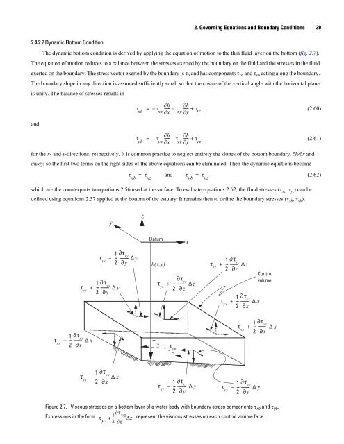
The dynamic bottom condition is derived by applying the equation of motion to the thin fluid layer on the bottom (fig. 2.7).
The equation of motion reduces to a balance between the stresses exerted by the boundary on the fluid and the stresses in the fluid
exerted on the boundary. The stress vector exerted by the boundary is τ b and has components τ xb and τ yb acting along the boundary.
The boundary slope in any direction is assumed sufficiently small so that the cosine of the vertical angle with the horizontal plane
is unity. The balance of stresses results in
and
τ xb
τ yb
∂h ∂h
= – τ ----- – τ ----- + τ
xx ∂x xy ∂y xz
(2.60)
τ -----
∂h ∂h
= – – τ ----- + τ (2.61)
yx ∂x yy ∂y yz
for the x- and y-directions, respectively. It is common practice to neglect entirely the slopes of the bottom boundary, ∂h/∂x and
∂h/∂y, so the first two terms on the right sides of the above equations can be eliminated. Then the dynamic equations become
τ xb
= τ and τ
xz
yb
= τ , (2.62)
yz
which are the counterparts to equations 2.56 used at the surface. To evaluate equations 2.62, the fluid stresses (τ xz, τ yz) can be
defined using equations 2.57 applied at the bottom of the estuary. It remains then to define the boundary stresses (τ xb, τ yb).
τ xx
τ yy
1
--
2
τ ∂ xx
– -------- Δ x
∂ x
τ yx
τ xy
y
1
--
2
τ ∂
yy
+ -------- Δ y
∂ y
1
--
2
τ ∂ yx
– -------- Δ x
∂ x
1
--
2
τ ∂
xy
+ -------- Δy
∂ y
z
Datum
h(x,y)
τ xb
τ yz
τ xy
x
1
--
2
τ ∂ yz
+ -------- Δ z
∂ z
τ yb
1
--
2
τ ∂ xy
– -------- Δ y
∂ y
τ xz
1
--
2
τ ∂ xz
+ -------- Δ z
∂ z
τ yx
τ yy
1
--
2
τ ∂ yx
+ -------- Δ x
∂ x
τ xx
1
--
2
τ ∂ yy
– -------- Δ y
∂ y
Control
volume
1
--
2
τ ∂ xx
+ -------- Δ x
∂ x
Figure 2.7. Viscous stresses on a bottom layer of a water body with boundary stress components τ xb and τ yb.
Expressions in the form 1
τ -- represent the viscous stresses on each control volume face.
yz 2
∂τ yz
+
---------- Δz
∂z