A Semi-Implicit, Three-Dimensional Model for Estuarine ... - USGS

32 A Semi-Implicit, Three-Dimensional Model for Estuarine Circulation
and
1
----ρ
0
p ∂
-----
∂y
1
----ρ
0
p ∂
a
-------- g
∂y
ζ ∂
----- g
∂y
1
=
ζ
∫∂ρ
+ + ----- ----- dz′ .
ρ
0
∂y
z
(2.48)
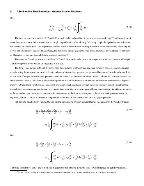
The integral terms in equations 2.47 and 2.48 are referred to as baroclinic terms and increase with depth 16 under most condi-
tions. Because the baroclinic terms require a complete specification of the density field, they couple the hydrodynamic solution to
the solution for the salt field. The importance of these terms accounts for the primary difference between modeling an estuary and
a river of homogeneous density. In an estuary, the horizontal density gradients often are an important driving force for the flow,
as illustrated for the longitudinal density gradients in figure 1.1.
The water surface slope terms in equations 2.47 and 2.48 are referred to as the barotropic terms and are constant with depth.
These incorporate the important driving force of the tide.
The terms in equations 2.47 and 2.48 involving the gradients of atmospheric pressure generally are neglected in estuarine
models, using the rationale that no significant gradients of atmospheric pressure are produced because of the relatively small size
of estuaries. Changes in atmospheric pressure cause the water level in most estuaries to adjust “coherently” (uniformly) over the
entire estuary. Normal variations in atmospheric pressure of ±20 millibars cause variations in estuarine water levels of approxi-
mately �20 cm; these variations are introduced into a numerical simulation through the open boundary conditions rather than
through the governing equations themselves. Gradients of atmospheric pressure generally are important only in wide-area models
of the coastal or open ocean when, for example, storm-surge predictions are attempted. If the atmospheric pressure terms are
neglected, it then is common to assume the pressure at the free surface corresponds to zero “gage” pressure.
and
Substituting equations 2.47 and 2.48, without the atmospheric pressure gradient terms, into equations 2.39 and 2.40 gives
∂u
∂uu
∂uv
∂uw
----- + -------- + -------- + --------- – fv g
∂t
∂x
∂y
∂z
ζ ∂
= – -----
∂x
g 1
ζ
∫∂ρ
∂
----- ----- dz′ ----- ⎛ ∂u
A ----- ⎞ ∂
----- ⎛ ∂u
ρ0 ∂x
∂x⎝
H A ----- ⎞ ∂ ∂u
–
+ + ----
∂x⎠
∂y⎝
H + ⎛A----- ⎞
∂y⎠
∂z⎝
V ∂z⎠
z
∂v
∂uv
∂vv
∂vw
---- + -------- + ------- + --------- + fu g
∂t
∂x
∂y
∂z
ζ ∂
= – -----
∂y
g 1
ζ
∫∂ρ
∂
----- ----- dz′ ----- ⎛ ∂v
A -----⎞
∂
----- ⎛ ∂v
ρ0 ∂x
∂x⎝
H A -----⎞
∂ ∂v
–
+ + ----
∂x⎠
∂y⎝
H + ⎛A----- ⎞
∂y⎠
∂z⎝
V .
∂z⎠
z
These are the forms of the x- and y-momentum equations that apply to estuarine tidal flows influenced by density variations.
16 For the case of a vertically well-mixed estuary, the density is independent of z and the baroclinic terms increase linearly with depth.
(2.49)
(2.50)