A Semi-Implicit, Three-Dimensional Model for Estuarine ... - USGS

More documents

Recommendations

Info

50 A Semi-Implicit, Three-Dimensional Model for Estuarine Circulation gradient, and Coriolis terms. The governing equations for use with orthogonal grids are significantly less complex that those for nonorthogonal grids, but they still include extra terms that represent the curvature of the coordinate system. Owing to the extra terms, the computational time that is required in solving the nonorthogonal curvilinear equations is approximately double that required for solving the Cartesian equations (Spaulding, 1984). Solving the orthogonal curvilinear equations requires approximately 25 percent greater computational time than the Cartesian equations (A.F. Blumberg, oral commun., 1995). Ideally the savings from any reduction in the number of grid points that is made possible by using a curvilinear model should be sufficient to compensate for the greater cost of the calculations for individual grid points. For a nonorthogonal curvilinear model in particular, that is not always possible. In these instances, the benefits from the greater flexibility in the placement of grid points using a nonorthogonal curvilinear model must outweigh the greater computational cost of the model, or a Cartesian or orthogonal-curvilinear model should be used. 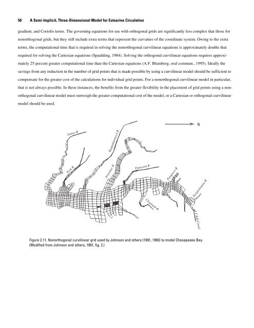James R York R Rappahannock R Potomac R Patuxent R Choptank R Patapsco R Figure 2.11. Nonorthogonal curvilinear grid used by Johnson and others (1991, 1993) to model Chesapeake Bay. (Modified from Johnson and others, 1991, fig. 2.) Susquehanna R C&D Canal N
2. Governing Equations and Boundary Conditions 51 Besides the increased complexity of the governing equations, the following additional drawbacks of models that are based on the curvilinear forms of the governing equations should be considered: 1. Considerable effort must be expended in defining the curvilinear grid transformation from computational to physical space. Generally, a numerical grid generator like the computer program EAGLE (Thompson and others, 1985) is needed to assign the spatial locations of the curvilinear grid points. For an orthogonal grid, the grid generation process is often iterative, continuing until a grid is found that reasonably approximates all boundaries of the domain while also satisfying the constraint equations for the orthogonality of intersecting grid lines. Reviews of grid generation techniques for fluid mechanics compu- tations are given by Eiseman (1985) and Hoffmann (1989). 2. Curvilinear models are not ideally suited for situations when the wetting and drying of boundary grid points occurs, as is common in estuarine tidal flats. In these situations, the estuarine boundary is in motion, and there is little likelihood that the boundary will be represented smoothly through all phases of the wetting and drying cycle. 3. When using curvilinear grids (especially strongly nonorthogonal ones), one must ensure that numerical dispersion errors are not introduced as waves propagate through regions of varying grid size and aspect ratio. Further studies of these errors are needed. 4. According to Wang (1992), a guaranteed conservative form of the advection terms does not exist for the horizontal momentum equations expressed with contravariant velocity components in a curvilinear, orthogonal or nonorthogonal, coordinate system. Although using a conservative form of the momentum advection terms in an estuarine model formulation is not always essential, it is usually desirable for the best possible behavior of the numerical model. The model described in this report will use Cartesian horizontal coordinates only. As can be concluded from this discussion, for cases in which a reasonably uniform grid resolution is appropriate and when precise boundary fitting is not important (because, for example, boundary areas have very low velocities or are subject to wetting and drying cycles), Cartesian models are preferred for their efficiency, convenience, and generally superior numerical behavior. In any case, solving the Cartesian form of equations should always be the first step in developing and testing a new model, as is the case herein. 2.6.2 Vertical Coordinate Transformations Three-dimensional models that are based upon a layered or grid-box approach in the vertical direction generally use one of three types of vertical coordinate systems. The first is a standard z-coordinate, or level-plane, system that has been used in the equations derived so far. Using z-coordinates, the governing equations are solved on a vertical grid system that is composed of horizontal layers with exchanges of mass, momentum, and salt taking place between the layers. The position of the layers is fixed ver- tically. The details of schematizing the governing equations using a z-coordinate layering system are presented in Chapters 3 and 4.
Page 1:
In cooperation with the Interagency
Page 4 and 5:
U.S. Department of the Interior Dir
Page 6 and 7:
This page intentionally left blank.
Page 8 and 9:
vi 4.2 Semi-Implicit One-Dimensiona
Page 10 and 11:
viii Figure 5.6. Graph showing solu
Page 12 and 13:
x Tables Table 2.1. Dimensionless n
Page 14 and 15: This page intentionally left blank.
Page 16 and 17: 2 A Semi-Implicit, Three-Dimensiona
Page 24 and 25: 10 A Semi-Implicit, Three-Dimension
Page 48 and 49: 2.4.1.2 Dynamic Surface Condition 2
Page 68 and 69: Water surface Water surface Level p
Page 70 and 71: h 1 h 2 h 3 h 4 h 5 h 6 z 1 ⁄ 2 z
Page 114 and 115:
100 A Semi-Implicit, Three-Dimensio
Page 116 and 117:
Page 118 and 119:
Page 120 and 121:
Page 122 and 123:
Page 124 and 125:
Page 126 and 127:
Page 128 and 129:
Page 130 and 131:
Page 132 and 133:
Page 134 and 135:
Page 136 and 137:
Page 138 and 139:
Page 140 and 141:
Page 142 and 143:
Page 144 and 145:
Page 146 and 147:
Page 148 and 149:
Page 150 and 151:
Page 152 and 153:
Page 154 and 155:
Page 156 and 157:
Page 158 and 159:
Page 160 and 161:
Page 162 and 163:
Page 164 and 165:
Page 166 and 167:
Page 168 and 169:
Page 170 and 171:
Page 172 and 173:
Page 174 and 175:
Page 176 and 177:
Page 178 and 179:
Page 180 and 181:
Page 182 and 183:
Page 184 and 185:
Page 186 and 187:
Page 188 and 189:
Page 190:
show all

A Semi-Implicit, Three-Dimensional Model for Estuarine ... - USGS

You also want an ePaper? Increase the reach of your titles

Delete template?

Save as template?