A Semi-Implicit, Three-Dimensional Model for Estuarine ... - USGS

96 A Semi-Implicit, Three-Dimensional Model for Estuarine Circulation
5.2.1.1 Two-Level Scheme
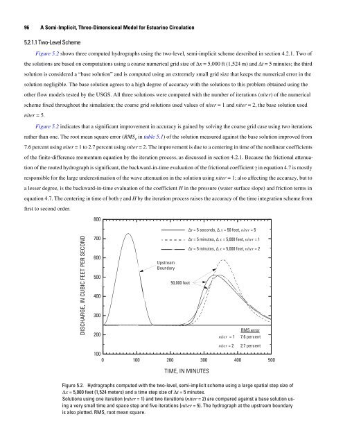
Figure 5.2 shows three computed hydrographs using the two-level, semi-implicit scheme described in section 4.2.1. Two of
the solutions are based on computations using a coarse numerical grid size of Δx = 5,000 ft (1,524 m) and Δt = 5 minutes; the third
solution is considered a “base solution” and is computed using an extremely small grid size that keeps the numerical error in the
solution negligible. The base solution agrees to a high degree of accuracy with the solutions to this problem obtained using the
other flow models tested by the USGS. All three solutions were computed with the number of iterations (niter) of the numerical
scheme fixed throughout the simulation; the coarse grid solutions used values of niter = 1 and niter = 2, the base solution used
niter = 5.
Figure 5.2 indicates that a significant improvement in accuracy is gained by solving the coarse grid case using two iterations
rather than one. The root mean square error (RMS e in table 5.1) of the solution measured against the base solution improved from
7.6 percent using niter = 1 to 2.7 percent using niter = 2. The improvement is due to a centering in time of the nonlinear coefficients
of the finite-difference momentum equation by the iteration process, as discussed in section 4.2.1. Because the frictional attenua-
tion of the routed hydrograph is significant, the backward-in-time evaluation of the frictional coefficient γ in equation 4.7 is mostly
responsible for the large underestimation of the wave attenuation in the solution using niter = 1; also affecting the accuracy, but to
a lesser degree, is the backward-in-time evaluation of the coefficient H in the pressure (water surface slope) and friction terms in
equation 4.7. The centering in time of both γ and H by the iteration process raises the accuracy of the time integration scheme from
first to second order.
DISCHARGE, IN CUBIC FEET PER SECOND
800
700
600
500
400
300
200
Upstream
Boundary
50,000 feet
100
0 100 200 300 400 500
TIME, IN MINUTES
Δt = 5 seconds, Δ x = 50 feet, niter = 5
Δt = 5 minutes, Δ x = 5,000 feet, niter = 1
Δt = 5 minutes, Δ x = 5,000 feet, niter = 2
RMS error
niter = 1 7.6 percent
niter = 2
2.7 percent
Figure 5.2. Hydrographs computed with the two-level, semi-implicit scheme using a large spatial step size of
Δx = 5,000 feet (1,524 meters) and a time step size of Δt = 5 minutes.
Solutions using one iteration (niter = 1) and two iterations (niter = 2) are compared against a base solution using
a very small time and space step and five iterations (niter = 5). The hydrograph at the upstream boundary
is also plotted. RMS, root mean square.