A Semi-Implicit, Three-Dimensional Model for Estuarine ... - USGS

112 A Semi-Implicit, Three-Dimensional Model for Estuarine Circulation
As seen in figures 5.9 and 5.10, the leapfrog scheme 46 solution to the hydrograph problem produces errors much smaller than
those produced by the two-level scheme without iteration (niter = 1) shown in figures 5.4 and 5.7. By involving three time levels
in the finite-difference equations, the leapfrog scheme achieves second-order accuracy in the time integration by evaluating the
nonlinear coefficients γ and H in equation and the advection term in equation 4.14, at the time level n, which is centered between
levels n + 1 and n – 1 (fig.4.3). As pointed out previously, the solutions to this test problem are particularly sensitive to the
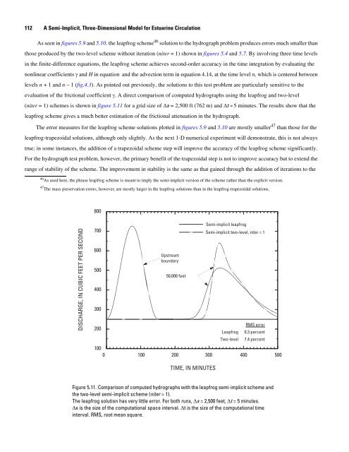
evaluation of the frictional coefficient γ. A direct comparison of computed hydrographs using the leapfrog and two-level
(niter = 1) schemes is shown in figure 5.11 for a grid size of Δx = 2,500 ft (762 m) and Δt = 5 minutes. The results show that the
leapfrog scheme gives a much better estimation of the frictional attenuation in the hydrograph.
The error measures for the leapfrog scheme solutions plotted in figures 5.9 and 5.10 are mostly smaller 47 than those for the
leapfrog-trapezoidal solutions, although only slightly. As the next 1-D numerical experiment will demonstrate, this is not always
true; in some instances, the addition of a trapezoidal scheme step will improve the accuracy of the leapfrog scheme significantly.
For the hydrograph test problem, however, the primary benefit of the trapezoidal step is not to improve accuracy but to extend the
range of stability of the scheme. The improvement in stability is the same as that gained through the addition of iterations to the
46 As used here, the phrase leapfrog scheme is meant to imply the semi-implicit version of the scheme rather than the explicit version.
47 The mass preservation errors, however, are mostly larger in the leapfrog solutions than in the leapfrog-trapezoidal solutions.
DISCHARGE, IN CUBIC FEET PER SECOND
800
700
600
500
400
300
200
Upstream
boundary
50,000 feet
Semi-implicit leapfrog
Semi-implicit two-level, niter = 1
RMS error
Leapfrog 0.3 percent
Two-level 7.4 percent
100
0 100 200 300 400 500
TIME, IN MINUTES
Figure 5.11. Comparison of computed hydrographs with the leapfrog semi-implicit scheme and
the two-level semi-implicit scheme (niter = 1).
The leapfrog solution has very little error. For both runs, Δx = 2,500 feet, Δt = 5 minutes.
Δx is the size of the computational space interval. Δt is the size of the computational time
interval. RMS, root mean square.