A Semi-Implicit, Three-Dimensional Model for Estuarine ... - USGS

78 A Semi-Implicit, Three-Dimensional Model for Estuarine Circulation
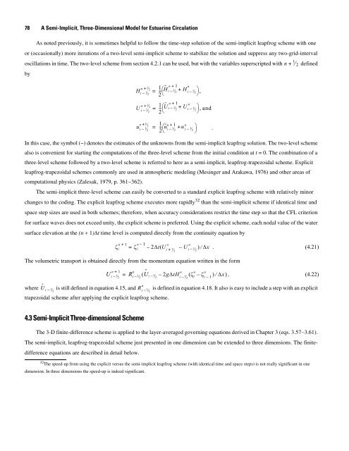
As noted previously, it is sometimes helpful to follow the time-step solution of the semi-implicit leapfrog scheme with one
or (occasionally) more iterations of a two-level semi-implicit scheme to stabilize the solution and suppress any two-grid-interval
oscillations in time. The two-level scheme from section 4.2.1 can be used, but with the variables superscripted with n
by
+ ⁄ 1
-- H
2
˜ n + 1 n
i – 1 = ⎛ ⁄ + H 2 i – 1 ⎞
⁄ 2 ,
⎝ ⎠
n 1
2 Hi – 1⁄ 2
n
+ ⁄ 1 + 1 n
-- Ũ i – 1 = ⎛ ⁄ + U 2 i – 1 ⎞
⁄ 2 , and
2⎝
⎠
n 1
2 U i – 1⁄ 2
+ ⁄ 1 n -- + 1 n
= ⎛ũi– 1
2 2 ⁄ + u i – 1 ⎞
⁄ 2 .
⎝ ⎠
n 1
2 ui – 1⁄ 2
1
+ ⁄ 2 defined
In this case, the symbol (~) denotes the estimates of the unknowns from the semi-implicit leapfrog solution. The two-level scheme
also is convenient for starting the computations of the three-level scheme from the initial condition at t = 0. The combination of a
three-level scheme followed by a two-level scheme is referred to here as a semi-implicit, leapfrog-trapezoidal scheme. Explicit
leapfrog-trapezoidal schemes commonly are used in atmospheric modeling (Mesinger and Arakawa, 1976) and other areas of
computational physics (Zalesak, 1979, p. 361−362).
The semi-implicit three-level scheme can easily be converted to a standard explicit leapfrog scheme with relatively minor
changes to the coding. The explicit leapfrog scheme executes more rapidly 32 than the semi-implicit scheme if identical time and
space step sizes are used in both schemes; therefore, when accuracy considerations restrict the time step so that the CFL criterion
for surface waves does not exceed unity, the explicit scheme is preferred. Using the explicit scheme, each nodal value of the water
surface elevation at the (n + 1)Δt time level is computed directly from the continuity equation by
n + 1
ζi n – 1
n
n
= ζ i – ( + – U
⁄ i – 1⁄ ) ⁄ Δx.
(4.21)
2
2Δt U i 1 2
The volumetric transport is obtained directly from the momentum equation written in the form
+
n 1
U i – 1⁄ 2
n
Ri – 1⁄ Û 2 i 1⁄ 2
n
where Û i – 1⁄ is still defined in equation 4.15, and R 2
i – 1⁄ 2
trapezoidal scheme after applying the explicit leapfrog scheme.
4.3 Semi-Implicit Three-dimensional Scheme
n n n
= ( – – 2gΔtHi – 1⁄ ( ζi – ζ
2 i – 1)
⁄ Δx)
, (4.22)
is defined in equation 4.18. It also is easy to include a step with an explicit
The 3-D finite-difference scheme is applied to the layer-averaged governing equations derived in Chapter 3 (eqs. 3.57−3.61).
The semi-implicit, leapfrog-trapezoidal scheme just presented in one dimension can be extended to three dimensions. The finite-
difference equations are described in detail below.
32 The speed-up from using the explicit versus the semi-implicit leapfrog scheme (with identical time and space steps) is not really significant in one
dimension. In three dimensions the speed-up is indeed significant.