A Semi-Implicit, Three-Dimensional Model for Estuarine ... - USGS

More documents

Recommendations

Info

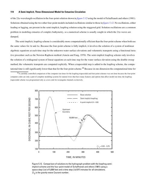
114 A Semi-Implicit, Three-Dimensional Model for Estuarine Circulation of the 2Δx-wavelength oscillation in the four-point solution shown in figure 5.12 using the model of Schaffranek and others (1981). Solutions obtained using the two other four-point models included oscillations similar to those in figure 5.12. No oscillations, either leading or lagging, are present in the semi-implicit, leapfrog solution using the staggered grid. Solution oscillations are a common problem in modeling estuaries of complex bathymetry, so a numerical scheme is usually sought in which the 2Δx waves are damped. The semi-implicit, leapfrog scheme is considerably more computationally efficient than the four-point scheme when both use the same values for Δt and Δx. Because the four-point scheme is fully implicit, it involves the solution of a system of nonlinear algebraic equations at each time step for the unknown water surface elevations and volumetric transports using a functional itera- tive procedure such as the Newton-Raphson method (Amein and Fang, 1970). The semi-implicit leapfrog scheme only involves the solution of a tridiagonal system of linear equations at each time step for the water surface elevation using the double-sweep method; the volumetric transports are computed explicitly. When a trapezoidal step is added to the leapfrog scheme, the computational time is still significantly lower than that for the four-point scheme. 48 Because in one dimension the computational time for 48 A carefully controlled comparison of the computer run times for the leapfrog-trapezoidal and four-point schemes was not done because the four-point computer codes are only a part of complete modeling systems for natural rivers that have many features and options that affect model run time; the leapfrog- trapezoidal scheme was programmed only as a test code for rectangular channels exclusively. DISCHARGE, IN CUBIC FEET PER SECOND 800 700 600 500 400 300 200 Upstream boundary 50,000 feet Crg = 0.53 – 0.75 100 0 100 200 300 400 500 TIME, IN MINUTES Base solution Semi-implicit leapfrog 4-point implicit (θ = 0.6) Figure 5.12. Comparison of solutions to the hydrograph problem with the leapfrog semiimplicit scheme and the four-point model of Schaffranek and others (1981) using a space step (Δx) of 5,000 feet and a time step (Δt) 0f 5 minutes for all simulations. Cr g is the gravity-wave Courant number.
5. Numerical Experiments 115 a numerical scheme generally is not too important in choosing a scheme, the four-point scheme is sometimes preferred over other schemes for the convenience of the fully dense grid and the ease with which the compact four-point computational stencil allows the space interval Δx to be varied between node points without affecting the accuracy of the approximation. In one dimension, staggered grid schemes are in general not as well suited to irregular Δx distance intervals as the four-point scheme. In three dimen- sions, however, the computational run time of a multidimensional four-point scheme would be prohibitively long for most real applications, and the semi-implicit scheme clearly is a better choice for reasons of computational efficiency. Flexibility in the hor- izontal grid point placement in a 3-D model can be achieved using a coordinate transformation, which is easily accommodated with a semi-implicit scheme, as demonstrated in the 3-D, curvilinear-coordinate model of Muin and Spaulding (1997a). 5.2.2 Tidal Flow in a Closed Channel The second 1-D numerical experiment uses a variation of a problem suggested by Alan F. Blumberg (written commun., 1992) to test the numerical damping characteristics of a hydrodynamic model. It is the propagation of a tidal wave from the sea into a wide rectangular channel that is closed at the landward boundary (fig. 5.13). The channel is 315,000 ft (96 km) long and filled with water initially at rest (Q 0 = 0) to a uniform depth H 0 = 33 ft (10 m). The channel is wide in comparison with the depth of water, so the simulations are based on a unit width. The Manning resistance coefficient for the channel is n = 0.020. H 0 Sea Tidal forcing ζ = ζ (t) Datum Channel characteristics B = 1 foot (unit width channel) L = 315,000 feet S 0 = 0.00 Manning’s n = 0.020 x L EXPLANATION Δ Wall Initial flow conditions Q 0 = 0.0 H 0 = 33 feet Figure 5.13. Channel characteristics and initial flow conditions for the 1-dimensional tidal test problem. The water in the channel is initially at rest at a uniform depth of H 0 . Tidal forcing is introduced at the seaward boundary causing the water surface to oscillate. Two successive positions of the water surface are shown. At the seaward boundary, water moves up and down and horizontally. At the wall boundary, water moves up and down only.
Page 1:
In cooperation with the Interagency
Page 4 and 5:
U.S. Department of the Interior Dir
Page 6 and 7:
This page intentionally left blank.
Page 8 and 9:
vi 4.2 Semi-Implicit One-Dimensiona
Page 10 and 11:
viii Figure 5.6. Graph showing solu
Page 12 and 13:
x Tables Table 2.1. Dimensionless n
Page 14 and 15:
This page intentionally left blank.
Page 16 and 17:
2 A Semi-Implicit, Three-Dimensiona
Page 18 and 19:
Page 20 and 21:
Page 22 and 23:
Page 24 and 25:
10 A Semi-Implicit, Three-Dimension
Page 26 and 27:
Page 28 and 29:
Page 30 and 31:
Page 32 and 33:
Page 34 and 35:
Page 36 and 37:
Page 38 and 39:
Page 40 and 41:
Page 42 and 43:
Page 44 and 45:
Page 46 and 47:
Page 48 and 49:
2.4.1.2 Dynamic Surface Condition 2
Page 50 and 51:
Page 52 and 53:
Page 54 and 55:
Page 56 and 57:
Page 58 and 59:
Page 60 and 61:
Page 62 and 63:
Page 64 and 65:
Page 66 and 67:
Page 68 and 69:
Water surface Water surface Level p
Page 70 and 71:
h 1 h 2 h 3 h 4 h 5 h 6 z 1 ⁄ 2 z
Page 72 and 73:
Page 74 and 75:
Page 76 and 77:
Page 78 and 79: 64 A Semi-Implicit, Three-Dimension
Page 114 and 115: 100 A Semi-Implicit, Three-Dimensio
Page 178 and 179:
164 A Semi-Implicit, Three-Dimensio
Page 180 and 181:
Page 182 and 183:
Page 184 and 185:
Page 186 and 187:
Page 188 and 189:
Page 190:
show all

A Semi-Implicit, Three-Dimensional Model for Estuarine ... - USGS

You also want an ePaper? Increase the reach of your titles

Delete template?

Save as template?