A Semi-Implicit, Three-Dimensional Model for Estuarine ... - USGS

74 A Semi-Implicit, Three-Dimensional Model for Estuarine Circulation
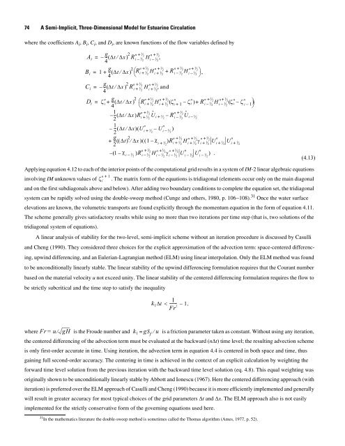
where the coefficients A i , B i , C i , and D i , are known functions of the flow variables defined by
A i
B i
C i
D i
g
– -- ( Δt ⁄ Δx )
4
2 n + 1⁄ 2 n + 1⁄ 2
=
R i – 1 Hi ⁄ 1
2 – ⁄ ,
2
g
1 -- ( Δt ⁄ Δx )
4
2 n + 1⁄ 2 n + 1⁄ 2 n + 1⁄ 2 n + 1⁄ 2
= + ⎛Ri+ 1⁄ H
2 i + 1⁄ + R
2 i – 1⁄ H ⎞
2 i – 1⁄ , 2
⎝ ⎠
g
– -- ( Δt ⁄ Δx )
4
2 n + 1⁄ 2 n + 1⁄ 2
=
R i + 1⁄ H
2 i + 1⁄ , and
2
n g
+ H i 1 2
+ H i 1 2
ζ i + -- ( Δt ⁄ Δx )
4
2 =
n 1
⎛ ⁄ 2 Ri + 1⁄ 2 ⎝
n + 1⁄ 2 n n n 1⁄ 2
+ ⁄ ( ζi + 1 – ζ i ) + R i – 1⁄ 2
n+ 1⁄ 2 n n
– ⁄ ( ζ i – ζ ⎞
i – 1)
⎠
1
n + 1⁄ 2
n + 1⁄ 2
– -- ( Δt ⁄ Δx )Ri1 2
+ ⁄ Û
2
i + 1⁄ – R 2 i – 1⁄ Û
2
i – 1⁄ 2
1
n
n
– -- ( Δt ⁄ Δx)
( U i 1
2
+ ⁄ – U
2 i – 1⁄ )
2
g
-- ( Δt)
2
( 1 – χ i – 1⁄ ) 2
n 1⁄ 2
– ⁄
n 1⁄ 2
– ⁄
n 1⁄ 2
– ⁄
n
– ⁄
n
– ⁄ ) .
2 n + 1
( ⁄ Δx ) 1 χ ⁄ 2 n + 1⁄ 2 n + 1⁄ 2 n n
+
( ( – i + 1⁄ )R
2 i + 1⁄ H
2 i + 1⁄ γ
2 i + 1⁄ U
2 i + 1⁄ U
2 i + 1⁄ 2
+ + +
– R i 1 H
2 i 1 γ
2 i 1 U
2 i 1 U
2 i 1
2
Applying equation 4.12 to each of the interior points of the computational grid results in a system of IM-2 linear algebraic equations
n + 1
involving IM unknown values of ζ i . The matrix form of the equations is tridiagonal (elements occur only on the main diagonal
and on the first subdiagonals above and below). After adding two boundary conditions to complete the equation set, the tridiagonal
system can be rapidly solved using the double-sweep method (Cunge and others, 1980, p. 106−108). 31 Once the water surface
elevations are known, the volumetric transports are found explicitly through the momentum equation in the form of equation 4.11.
The scheme generally gives satisfactory results while using no more than two iterations per time step (that is, two solutions of the
tridiagonal system of equations).
A linear analysis of stability for the two-level, semi-implicit scheme without an iteration procedure is discussed by Casulli
and Cheng (1990). They considered three choices for the explicit approximation of the advection term: space-centered differenc-
ing, upwind differencing, and an Eulerian-Lagrangian method (ELM) using linear interpolation. Only the ELM method was found
to be unconditionally linearly stable. The linear stability of the upwind differencing formulation requires that the Courant number
based on the material velocity u not exceed unity. The linear stability of the centered differencing formulation requires the flow to
be strictly subcritical and the time step to satisfy the inequality
k1Δt 1
Fr 2 < ------- – 1,
where Fr = u⁄ gH is the Froude number and k1 = gSf ⁄ u is a friction parameter taken as constant. Without using any iteration,
the centered differencing of the advection term must be evaluated at the backward (nΔt) time level; the resulting advection scheme
is only first-order accurate in time. Using iteration, the advection term in equation 4.4 is centered in both space and time, thus
gaining full second-order accuracy. The centering in time is achieved in the context of an explicit calculation by weighting the
forward time level solution from the previous iteration with the backward time level solution (eq. 4.8). This equal weighting was
originally shown to be unconditionally linearly stable by Abbott and Ionescu (1967). Here the centered differencing approach (with
iteration) is preferred over the ELM approach of Casulli and Cheng (1990) because it is more efficiently implemented and generally
will result in greater accuracy for most typical choices of the grid parameters Δt and Δx. The ELM approach also is not easily
implemented for the strictly conservative form of the governing equations used here.
31 In the mathematics literature the double-sweep method is sometimes called the Thomas algorithm (Ames, 1977, p. 52).
(4.13)