A Semi-Implicit, Three-Dimensional Model for Estuarine ... - USGS

52 A Semi-Implicit, Three-Dimensional Model for Estuarine Circulation
The second type of vertical coordinate system uses density to replace depth (z) as the vertical coordinate, making density an
independent variable in the transformed system (x, y, ρ, t). The coordinate z becomes a dependent variable that identifies the depth
at which the density is defined for a given x, y location and time t. The governing equations are schematized by using stacked layers
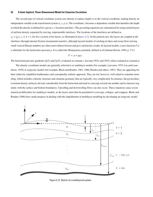
of uniform density separated by moving, impermeable interfaces. The locations of the interfaces are defined as
z k = ζ k (x, y, t), k = 1, km for a system of km layers, as illustrated in figure 2.12. In the general case, the layers are coupled at the
interfaces through internal friction (momentum transfer), although layered models of seiching in lakes and ocean flows having
small vertical Ekman numbers are often used without friction and give satisfactory results. In layered models, a new function P is
a substitute for the hydrostatic pressure p. It is called the Montgomery potential, defined as (Cushman-Roisin, 1994, p. 171)
P = p+ ρgz .
The horizontal pressure gradients ∂p/∂x and ∂p/∂y, evaluated at constant z, become ∂P/∂x and ∂P/∂y when evaluated at constant ρ.
The density-coordinate models are generally referred to as multilayer models (for example, Laevastu, 1975; Liu and Leen-
dertse, 1978) or isopycnic models (for example, Bleck and Boudra, 1981, 1986; Boudra and others, 1987). They are appealing for
their relatively simplified mathematics and conceptually realistic approach. They are not, however, well suited to estuarine mod-
eling, which includes a density structure and estuarine geometry that are typically very complicated. In estuaries, the pycnoclines
(constant density surfaces) deviate considerably from the horizontal and tend to converge toward one another and to intersect reg-
ularly with the surface and bottom boundaries. Upwelling and downwelling flows can also occur. These situations cause severe
numerical difficulties for multilayer models, as the layers must then be permitted to converge, collapse, and reappear. Bleck and
Boudra (1986) have made progress in dealing with the impediments of multilayer modeling by developing an isopycnic model
z
y
x
ρ 1
ρ 2
.
.
.
ρ km
Figure 2.12. Sketch of a multilayered system.
ζ
ζ 1
ζ 2
ζ km–1
ζ km
k = 1
k = 2
=
–
k = km
h ( x , y )