A Semi-Implicit, Three-Dimensional Model for Estuarine ... - USGS

120 A Semi-Implicit, Three-Dimensional Model for Estuarine Circulation
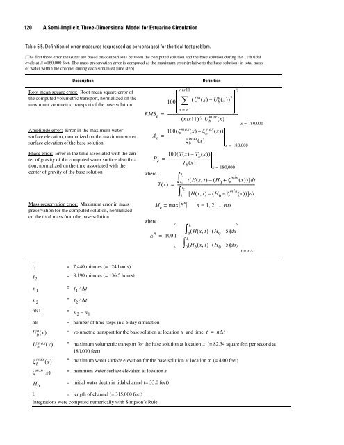
Table 5.5. Definition of error measures (expressed as percentages) for the tidal test problem.
[The first three error measures are based on comparisons between the computed solution and the base solution during the 11th tidal
cycle at x =180,000 feet. The mass preservation error is computed as the maximum error (relative to the base solution) in total mass
of water within the channel during each simulated time step]
Description Definition
Root mean square error: Root mean square error of
the computed volumetric transport, normalized on the
maximum volumetric transport of the base solution
Amplitude error: Error in the maximum water
surface elevation, normalized on the maximum water
surface elevation of the base solution
Phase error: Error in the time associated with the center
of gravity of the computed water surface distribution,
normalized on the time associated with the
center of gravity of the base solution
Mass preservation error: Maximum error in mass
preservation for the computed solution, normalized
on the total mass from the base solution
t 1 = 7,440 minutes (= 124 hours)
t 2
n 1
n 2
= 8,190 minutes (= 136.5 hours)
= t1 ⁄ Δt
= t2 ⁄ Δt
RMS e
A e
P e
where
nts11 = n2 – n1 nts = number of time steps in a 6 day simulation
n
Ub ( x)
nts11
∑
100
U n n
( ( x)
– Ub ( x)
) 2
n = n1
( nts11)
1 = ---------------------------------------------------------------------------
⁄ max 2 Ub ( x)
100 ζ max max
( ( x)
– ζb ( x)
)
= ---------------------------------------------------------max
ζb ( x)
100( Tx ( ) – Tb( x)
)
= --------------------------------------------
Tb( x)
Tx ( )
M e
t2 ∫t1 t2 ∫t1 x = 180,000
1⁄ 2
x = 180,000
x = 180,000
tHxt ( , ) H0 ζ min [ – ( + ( x)
) ]dt
Hxt ( , ) H0 ζ min = ----------------------------------------------------------------------------------
[ – ( + ( x)
) ]dt
max E n
= n = 1, 2 , ... , nts
= volumetric transport for the base solution at location x and time t = nΔt
Umax b ( x)
= maximum volumetric transport for the base solution at location x (= 82.34 square feet per second at
180,000 feet)
max
ζb ( x)
= maximum water surface elevation for the base solution at location x (= 4.00 feet)
ζ min ( x)
= minimum water surface elevation at location x
H0 = initial water depth in tidal channel (= 33.0 feet)
L = length of channel (= 315,000 feet)
Integrations were computed numerically with Simpson’s Rule.
where
E n
=
⎛ L
⎞
⎜ ∫0( Hxt ( , ) – ( H0 – 5)
)dx⎟
100⎜1– -------------------------------------------------------- ⎟
L
⎜ ⎟
⎝ ( Hb( x, t)
– ( H0 – 5)
)dx⎠
∫ 0
t = nΔt