A Semi-Implicit, Three-Dimensional Model for Estuarine ... - USGS

70 A Semi-Implicit, Three-Dimensional Model for Estuarine Circulation
Continuity,
x-Momentum,
∂U
-------
∂t
∂ζ
------
∂t
∂U
+ ------- = 0 ; (4.1)
∂x
∂uU
---------- gH
∂x
∂ζ
+ + ----- = – gHSf .
(4.2)
∂x
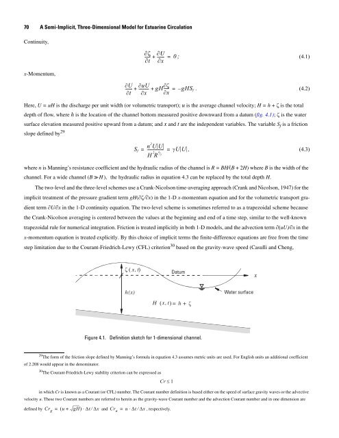
Here, U = uH is the discharge per unit width (or volumetric transport); u is the average channel velocity; H = h + ζ is the total
depth of flow, where h is the location of the channel bottom measured positive downward from a datum (fig. 4.1); ζ is the water
surface elevation measured positive upward from a datum; and x and t are the independent variables. The variable Sf is a friction
slope defined by 29
S f
n 2 UU
= ----------------- = γU U , (4.3)
H 2
R 4 ⁄ 3
where n is Manning’s resistance coefficient and the hydraulic radius of the channel is R = BH⁄(B + 2H) where B is the width of the
channel. For a wide channel (B >> H ), the hydraulic radius in equation 4.3 can be replaced by the total depth H.
The two-level and the three-level schemes use a Crank-Nicolson time-averaging approach (Crank and Nicolson, 1947) for the
implicit treatment of the pressure gradient term gH(∂ζ ⁄∂x) in the 1-D x-momentum equation and for the volumetric transport gra-
dient term ∂U⁄∂x in the 1-D continuity equation. The two-level scheme is sometimes referred to as a trapezoidal scheme because
the Crank-Nicolson averaging is centered between the values at the beginning and end of a time step, similar to the well-known
trapezoidal rule for numerical integration. Friction is treated implicitly in both 1-D models, and the advection term ∂(uU)⁄∂x in the
x-momentum equation is treated explicitly. By this choice of implicit terms the finite-difference equations are free from the time
step limitation due to the Courant-Friedrich-Lewy (CFL) criterion 30 based on the gravity-wave speed (Casulli and Cheng,
ζ ( x, t)
h(x)
Figure 4.1. Definition sketch for 1-dimensional channel.
29 The form of the friction slope defined by Manning’s formula in equation 4.3 assumes metric units are used. For English units an additional coefficient
of 2.208 would appear in the denominator.
30The Courant-Friedrich-Lewy stability criterion can be expressed as
H ( x, t)
= h + ζ
Cr ≤ 1
in which Cr is known as a Courant (or CFL) number. The Courant number definition is based either on the speed of surface gravity waves or the advective
velocity u. These two Courant numbers are referred to herein as the gravity-wave Courant number and the advection Courant number and in one dimension are
defined by Crg = ( u + gH)
⋅ Δt⁄ Δx and Cra = u ⋅ Δt ⁄ Δx,
respectively.
/
Datum
Water surface
x