A Semi-Implicit, Three-Dimensional Model for Estuarine ... - USGS

More documents

Recommendations

Info

32 A Semi-Implicit, Three-Dimensional Model for Estuarine Circulation and 1 ----ρ 0 p ∂ ----- ∂y 1 ----ρ 0 p ∂ a -------- g ∂y ζ ∂ ----- g ∂y 1 = ζ ∫∂ρ + + ----- ----- dz′ . ρ 0 ∂y z (2.48) The integral terms in equations 2.47 and 2.48 are referred to as baroclinic terms and increase with depth 16 under most conditions. Because the baroclinic terms require a complete specification of the density field, they couple the hydrodynamic solution to the solution for the salt field. The importance of these terms accounts for the primary difference between modeling an estuary and a river of homogeneous density. In an estuary, the horizontal density gradients often are an important driving force for the flow, as illustrated for the longitudinal density gradients in figure 1.1. The water surface slope terms in equations 2.47 and 2.48 are referred to as the barotropic terms and are constant with depth. These incorporate the important driving force of the tide. The terms in equations 2.47 and 2.48 involving the gradients of atmospheric pressure generally are neglected in estuarine models, using the rationale that no significant gradients of atmospheric pressure are produced because of the relatively small size of estuaries. Changes in atmospheric pressure cause the water level in most estuaries to adjust “coherently” (uniformly) over the entire estuary. Normal variations in atmospheric pressure of ±20 millibars cause variations in estuarine water levels of approxi- mately �20 cm; these variations are introduced into a numerical simulation through the open boundary conditions rather than through the governing equations themselves. Gradients of atmospheric pressure generally are important only in wide-area models of the coastal or open ocean when, for example, storm-surge predictions are attempted. If the atmospheric pressure terms are neglected, it then is common to assume the pressure at the free surface corresponds to zero “gage” pressure. and Substituting equations 2.47 and 2.48, without the atmospheric pressure gradient terms, into equations 2.39 and 2.40 gives ∂u ∂uu ∂uv ∂uw ----- + -------- + -------- + --------- – fv g ∂t ∂x ∂y ∂z ζ ∂ = – ----- ∂x g 1 ζ ∫∂ρ ∂ ----- ----- dz′ ----- ⎛ ∂u A ----- ⎞ ∂ ----- ⎛ ∂u ρ0 ∂x ∂x⎝ H A ----- ⎞ ∂ ∂u – + + ---- ∂x⎠ ∂y⎝ H + ⎛A----- ⎞ ∂y⎠ ∂z⎝ V ∂z⎠ z ∂v ∂uv ∂vv ∂vw ---- + -------- + ------- + --------- + fu g ∂t ∂x ∂y ∂z ζ ∂ = – ----- ∂y g 1 ζ ∫∂ρ ∂ ----- ----- dz′ ----- ⎛ ∂v A -----⎞ ∂ ----- ⎛ ∂v ρ0 ∂x ∂x⎝ H A -----⎞ ∂ ∂v – + + ---- ∂x⎠ ∂y⎝ H + ⎛A----- ⎞ ∂y⎠ ∂z⎝ V . ∂z⎠ z These are the forms of the x- and y-momentum equations that apply to estuarine tidal flows influenced by density variations. 16 For the case of a vertically well-mixed estuary, the density is independent of z and the baroclinic terms increase linearly with depth. (2.49) (2.50)
2.4 Boundary Conditions 2. Governing Equations and Boundary Conditions 33 To complete the system of mean-flow equations introduced in section 2.3, it is necessary to specify the boundary conditions for an estuarine flow. For a 3-D model application, boundary conditions must be specified at the free surface, bottom, shoreline, and open boundaries of the estuary. In this report, it is assumed that all boundaries other than the free surface are fixed and do not change with time. This eliminates any consideration of vertical movement of the bottom profile caused by sediment transport or the lateral movement of shoreline boundaries caused by wetting and drying of tidal flats. The treatment of these moving boundaries involves topics that are outside the scope of this report. It also is assumed that the estuary bottom is impermeable and that the effects of precipitation and evaporation at the free surface are negligible. The 3-D model test cases included in this report do not involve open boundaries, so the formulation of a generalized open boundary condition is not discussed here. It is recognized, however, that the proper specification of open boundary conditions is a challenging problem in modeling. 2.4.1 Free Surface Hydrodynamic boundary conditions at the free surface require that kinematic and dynamic conditions be satisfied. These conditions are discussed below. The boundary condition for the salt transport equation requires zero salt flux (∂s/∂z = 0) at the free surface. 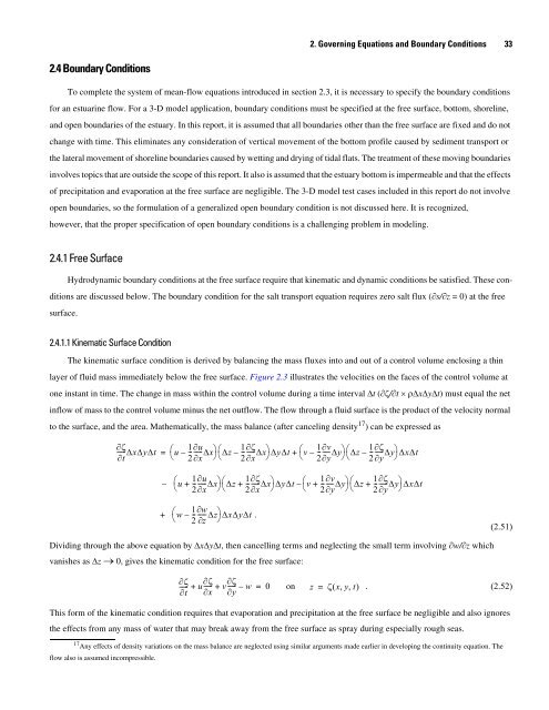2.4.1.1 Kinematic Surface Condition The kinematic surface condition is derived by balancing the mass fluxes into and out of a control volume enclosing a thin layer of fluid mass immediately below the free surface. Figure 2.3 illustrates the velocities on the faces of the control volume at one instant in time. The change in mass within the control volume during a time interval Δt (∂ζ/∂t × ρΔxΔyΔt) must equal the net inflow of mass to the control volume minus the net outflow. The flow through a fluid surface is the product of the velocity normal to the surface, and the area. Mathematically, the mass balance (after canceling density 17 ) can be expressed as ∂ζ 1 -----ΔxΔyΔt u -- ∂t 2 ∂u ⎛ – -----Δx ⎞ 1 Δz -- ⎝ ∂x ⎠ 2 ∂ζ ⎛ – -----Δx ⎞ 1 ΔyΔt v -- ⎝ ∂x ⎠ 2 ∂v ⎛ – ----- Δy⎞ 1 Δz -- ⎝ ∂y ⎠ 2 ∂ζ = + ⎛ – -----Δy ⎞ΔxΔt ⎝ ∂y ⎠ 1 u -- 2 ∂u ⎛ + -----Δx ⎞ 1 Δz -- ⎝ ∂x ⎠ 2 ∂ζ ⎛ + -----Δx ⎞ 1 – ΔyΔt v -- ⎝ ∂x ⎠ 2 ∂v ⎛ + ----- Δy⎞ 1 Δz -- ⎝ ∂y ⎠ 2 ∂ζ – ⎛ + -----Δy ⎞ΔxΔt ⎝ ∂y ⎠ + w 1 -- 2 w ∂ ⎛ – ------ Δz⎞ΔxΔyΔt . ⎝ ∂z ⎠ Dividing through the above equation by ΔxΔyΔt, then cancelling terms and neglecting the small term involving ∂w/∂z which vanishes as Δz → 0, gives the kinematic condition for the free surface: (2.51) ∂ζ ----- u ∂t ∂ζ ----- v ∂x ∂ζ + + ----- – w = 0 on z = ζ( x, y, t) . (2.52) ∂y This form of the kinematic condition requires that evaporation and precipitation at the free surface be negligible and also ignores the effects from any mass of water that may break away from the free surface as spray during especially rough seas. 17 Any effects of density variations on the mass balance are neglected using similar arguments made earlier in developing the continuity equation. The flow also is assumed incompressible.
Page 1: In cooperation with the Interagency
Page 4 and 5: U.S. Department of the Interior Dir
Page 6 and 7: This page intentionally left blank.
Page 8 and 9: vi 4.2 Semi-Implicit One-Dimensiona
Page 10 and 11: viii Figure 5.6. Graph showing solu
Page 12 and 13: x Tables Table 2.1. Dimensionless n
Page 14 and 15: This page intentionally left blank.
Page 16 and 17: 2 A Semi-Implicit, Three-Dimensiona
Page 24 and 25: 10 A Semi-Implicit, Three-Dimension
Page 48 and 49: 2.4.1.2 Dynamic Surface Condition 2
Page 68 and 69: Water surface Water surface Level p
Page 70 and 71: h 1 h 2 h 3 h 4 h 5 h 6 z 1 ⁄ 2 z
Page 96 and 97:
82 A Semi-Implicit, Three-Dimension
Page 98 and 99:
Page 100 and 101:
Page 102 and 103:
Page 104 and 105:
Page 106 and 107:
Page 108 and 109:
Page 110 and 111:
Page 112 and 113:
Page 114 and 115:
100 A Semi-Implicit, Three-Dimensio
Page 116 and 117:
Page 118 and 119:
Page 120 and 121:
Page 122 and 123:
Page 124 and 125:
Page 126 and 127:
Page 128 and 129:
Page 130 and 131:
Page 132 and 133:
Page 134 and 135:
Page 136 and 137:
Page 138 and 139:
Page 140 and 141:
Page 142 and 143:
Page 144 and 145:
Page 146 and 147:
Page 148 and 149:
Page 150 and 151:
Page 152 and 153:
Page 154 and 155:
Page 156 and 157:
Page 158 and 159:
Page 160 and 161:
Page 162 and 163:
Page 164 and 165:
Page 166 and 167:
Page 168 and 169:
Page 170 and 171:
Page 172 and 173:
Page 174 and 175:
Page 176 and 177:
Page 178 and 179:
Page 180 and 181:
Page 182 and 183:
Page 184 and 185:
Page 186 and 187:
Page 188 and 189:
Page 190:
show all

A Semi-Implicit, Three-Dimensional Model for Estuarine ... - USGS

You also want an ePaper? Increase the reach of your titles

Delete template?

Save as template?