A Semi-Implicit, Three-Dimensional Model for Estuarine ... - USGS

48 A Semi-Implicit, Three-Dimensional Model for Estuarine Circulation
Noye and Stevens (1987) used the same horizontal transformation as Boericke and Hall but solved the transformed governing
equations by using a nonuniform grid spacing in order to increase the grid resolution in regions of interest within the original coor-
dinate system. The nonuniform grid spacing in the computational space must be chosen according to certain criteria presented by
Noye and Stevens to retain the accuracy of the numerical approximations that are achievable for uniformly spaced grids. Because
the stretching coefficients are not constant in the method of Boericke and Hall, an additional term is introduced into the expression
for the transformed x-derivative.
To achieve even greater flexibility for the horizontal grid point placement than with stretched-coordinate models, curvilinear
coordinate models can be used. These models solve forms of the governing equations that are transformed into curvilinear coor-
dinates. The transformed equations can be solved on a rectangular grid, which is then transformed into a curvilinear grid in the
original coordinate system. The curvilinear grid is generally fitted to the physical boundary to avoid the stair-step patterns that
appear when curved boundaries are represented by conventional rectangular grids. Clustering grid points is possible in regions
where increased grid resolution is needed, such as navigation channels (Thompson and Johnson, 1986).
Curvilinear coordinate models have been developed that are based on horizontal grid transformations that are conformal (Reid
and others, 1977), generalized orthogonal (Willemse and others, 1985; Blumberg and Herring, 1987), and nonorthogonal (Johnson,
1982; Johnson and others, 1991; Sheng, 1986a; Spaulding, 1984; Spaulding and others, 1990; Muin and Spaulding, 1996). Con-
formal transformations are fully defined by analytic functions of a complex variable by using the techniques of conformal mapping
(Vallentine, 1967). Except at relatively few singular points, conformal grids are orthogonal: families of grid lines intersect perpen-
dicularly to one another. By the definition of a conformal transformation, the angles of the rectangular grid in computational space
are preserved in magnitude and sense under the transformation, which assures the orthogonality of the grid in the physical space.
For estuarine modeling, a generalized orthogonal curvilinear grid is usually preferred over a conformal grid because it allows a
more flexible spacing of grid lines; thus, for example, it is easy with a generalized orthogonal grid to choose grid lines that are
y
A B
Bx ( )
bx ( )
x
x = xˆ
yˆ = 1
y = b ( x ) + B ( x)yˆ
yˆ = 0
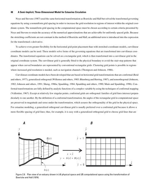
Figure 2.9. Plan view of an estuary shown in (A) physical space and (B) computational space using the transformation of
Boericke and Hall (1974).
yˆ
xˆ