A Semi-Implicit, Three-Dimensional Model for Estuarine ... - USGS
A Semi-Implicit, Three-Dimensional Model for Estuarine ... - USGS
A Semi-Implicit, Three-Dimensional Model for Estuarine ... - USGS
You also want an ePaper? Increase the reach of your titles
YUMPU automatically turns print PDFs into web optimized ePapers that Google loves.
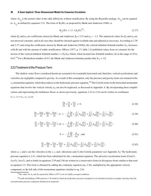
30 A <strong>Semi</strong>-<strong>Implicit</strong>, <strong>Three</strong>-<strong>Dimensional</strong> <strong>Model</strong> <strong>for</strong> <strong>Estuarine</strong> Circulation<br />
where D V0 is the neutral value of the eddy diffusivity without stratification. By using the Reynolds analogy, D V0 can be equated<br />
to A V0 as defined by equation 2.31. The <strong>for</strong>m of Φ s(Ri), as proposed by Munk and Anderson (1948), is<br />
Φ<br />
s<br />
( Ri)<br />
( 1 + β2Ri) α = 2 , (2.37)<br />
where β 2 and α 2 are coefficients chosen by Munk and Anderson: β 2 = 3.33 and α 2 = −1.5. The numerical values <strong>for</strong> β 2 and α 2 are<br />
not universal constants, and in all cases they should be checked against available data and adjusted as necessary. According to 2.29<br />
and 2.37 (and using the coefficients chosen by Munk and Anderson [1948]), the vertical turbulent Schmidt number Sc V increases<br />
with Ri and with the amount of stable stratification. Officer (1977, p. 17, table 1.2) published values from six estuaries <strong>for</strong> the<br />
inverse of the vertical turbulent Schmidt number ( = D V/A V) which, when inverted into Schmidt numbers, lie in the range of 10 to<br />
0.83. 14 For a Richardson number of 0.5, the Munk and Anderson <strong>for</strong>mulas predict that Sc V = 1.8.<br />
2.3.2 Treatment of the Pressure Term<br />
The shallow-water flows considered herein are assumed to be essentially horizontal and, there<strong>for</strong>e, vertical accelerations and<br />
velocities are negligible compared to gravity. As a result of this assumption, only the pressure and gravity terms are retained in the<br />
x 3 -momentum equation, which then reduces to the hydrostatic pressure equation. 15 The Coriolis terms in the horizontal momentum<br />
equations that involve the vertical velocity u 3 can also be neglected, as discussed in Appendix A. By incorporating these simplifi-<br />
cations and representing the turbulence fluxes as shown previously, equations 2.14 to 2.16 can be written in coordinates<br />
(x, y, z) = (x 1, x 2, x 3) as<br />
∂u<br />
∂v<br />
∂w<br />
----- + ---- + ------ = 0 , (2.38)<br />
∂x<br />
∂y<br />
∂z<br />
∂u<br />
∂uu<br />
∂uv<br />
∂uw<br />
1<br />
----- + -------- + -------- + --------- – fv -----<br />
∂t<br />
∂x<br />
∂y<br />
∂z<br />
ρ<br />
0<br />
p ∂ ∂<br />
----- ----- ⎛ ∂u<br />
A ----- ⎞ ∂<br />
----- ⎛ ∂u<br />
∂x<br />
∂x⎝<br />
H<br />
A ----- ⎞ ∂ ∂u<br />
= – + + ----<br />
∂x⎠<br />
∂y⎝<br />
H<br />
+ ⎛A----- ⎞<br />
∂y⎠<br />
∂z⎝<br />
V<br />
, (2.39)<br />
∂z⎠<br />
∂v<br />
∂uv<br />
∂vv<br />
∂vw<br />
1<br />
---- + -------- + ------- + --------- + fu -----<br />
∂t<br />
∂x<br />
∂y<br />
∂z<br />
ρ<br />
0<br />
p ∂ ∂<br />
----- ----- ⎛ ∂v<br />
A ----- ⎞ ∂<br />
----- ⎛ ∂v<br />
∂y<br />
∂x⎝<br />
H<br />
A ----- ⎞ ∂ ∂v<br />
= – + + ----<br />
∂x⎠<br />
∂y⎝<br />
H<br />
+ ⎛A-----⎞ ∂y⎠<br />
∂z⎝<br />
V , (2.40)<br />
∂z⎠<br />
0<br />
-----<br />
1<br />
ρ0 p ∂ ρ<br />
= – ----- – ----- g , and (2.41)<br />
∂z<br />
ρ0 ∂s<br />
∂us<br />
∂vs<br />
∂ws<br />
---- + ------- + ------- + -------- -----<br />
∂ ⎛D----- ∂s⎞<br />
-----<br />
∂ ⎛<br />
∂t<br />
∂x<br />
∂y<br />
∂z<br />
∂x⎝<br />
H<br />
D -----<br />
∂s⎞<br />
----<br />
∂ ∂s<br />
= +<br />
∂x⎠<br />
∂y⎝<br />
H<br />
+ ⎛D---- ⎞<br />
∂y⎠<br />
∂z⎝<br />
V , (2.42)<br />
∂z⎠<br />
where u, v, and w are the velocities in the x, y, and z directions and f is the Coriolis parameter (see Appendix A). The hydrostatic<br />
pressure equation is 2.41, which has been substituted <strong>for</strong> the z-momentum equation. The advective acceleration terms (∂uu/∂x,<br />
∂uv/∂y, ∂uw/∂z, and so <strong>for</strong>th) in equations 2.39 and 2.40 are written in a conservative <strong>for</strong>m (or divergence from) similar to that used<br />
in equation 2.5. This <strong>for</strong>m is obtained by adding the continuity equation (eq. 2.38), multiplied by the appropriate velocity<br />
component, to the left side of the momentum equations (similar to eq. 2.6).<br />
14 The values <strong>for</strong> AV and D V reported by Officer (1977) were <strong>for</strong> tidally averaged conditions.<br />
15 Casulli and Stelling (1996) present a 3-D model in which the hydrostatic pressure assumption is not introduced and give examples showing when the<br />
non-hydrostatic pressure component should not be neglected.


