A Semi-Implicit, Three-Dimensional Model for Estuarine ... - USGS

More documents

Recommendations

Info

46 A Semi-Implicit, Three-Dimensional Model for Estuarine Circulation In contrast to the momentum equation, the advective transport terms in the salt equation are very significant (table 2.3) and should be evaluated carefully in a numerical model to avoid artificial diffusion or spurious oscillations of the salt concentration field. Péclet numbers as large as those in table 2.1 indicate that estuarine flows are “advection dominated,” meaning that the transport of salt (and generally other solutes) is mostly by advection by the water currents and not by turbulent diffusion. The diffusion terms in the salt transport equation, however, should not be neglected. The accurate modeling of the vertical diffusion of salt is essential in a stratified estuary if the vertical profile of salinity is to be reproduced accurately. The modeling of horizontal salt diffusion may be less highly refined than the vertical diffusion in most estuaries, but it is still required to determine the proper horizontal distribution of salt. Quite often the size of the horizontal numerical grid used in estuarine modeling is large. All the horizontal advective motions acting over smaller scales than the grid are not resolved directly by the model but are considered to be mixing, and they must be represented by the horizontal diffusion terms. For this reason, the horizontal eddy diffusion coefficient, D H, is partly based on the size of the smallest eddies that are resolved by a model. 2.6 Coordinate Transformations The 3-D equations presented so far are written in standard Cartesian or rectangular coordinates. 20 Thus, the equations have a relatively simple form. When using the finite-difference method, the Cartesian equations generally are solved on a square or rectangular grid. The calculations can be very efficient because the simple form of the equations and the uniform grid system are con- venient for the implementation of most numerical schemes. Over the last two decades, however, it has become increasingly com- mon to transform the governing equations into other coordinate systems that allow variable or curvilinear grids to be used with greater flexibility in representing curved shoreline and bottom boundaries smoothly, or for resolving interior regions of interest using a higher density of grid points. The transformations can involve the horizontal coordinates or the vertical coordinate or both. Horizontal coordinate transformations are used almost exclusively in transforming the governing equations for finite-difference solution methods. Finite-element and finite-volume methods allow one to work with irregular grid systems without transforming the coordinates of the governing equations. It is also possible to use irregular (usually triangular) grids with finite-difference methods (see, for example, Thacker, 1977), but coordinate transformations are more commonly used. A brief review of the horizontal and vertical coordinate transformations in use today [1997] for estuarine and coastal modeling follows. 20 If a circulation model is to be applied to regions of the ocean having substantial variations in latitude (generally greater than a few tens of degrees), then the governing equations in rectangular coordinates are not appropriate. Spherical coordinates must be used to consider the curvature of the earth’s surface. For the relatively small horizontal scale of most estuaries, the use of rectangular coordinates introduces negligible errors.
2.6.1 Horizontal Coordinate Transformations 2. Governing Equations and Boundary Conditions 47 The simplest of horizontal coordinate transformations are those that stretch coordinates to form a numerical grid that is rectangular but not uniform. The transformation used by Butler (1978, 1980), and also implemented in the 3-D model by Sheng (1983), takes the form x axbxxˆ c = + x , y aybyyˆ c = + y , (2.72) where a x, b x, c x, a y, b y, and c y are arbitrarily chosen stretching coefficients. The governing equations are usually solved on a rectangular grid with square grid boxes after being transformed into the new coordinates xˆ , yˆ . 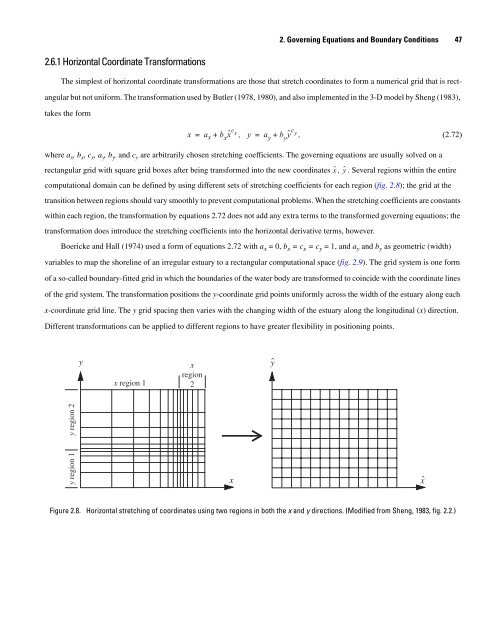Several regions within the entire computational domain can be defined by using different sets of stretching coefficients for each region (fig. 2.8); the grid at the transition between regions should vary smoothly to prevent computational problems. When the stretching coefficients are constants within each region, the transformation by equations 2.72 does not add any extra terms to the transformed governing equations; the transformation does introduce the stretching coefficients into the horizontal derivative terms, however. Boericke and Hall (1974) used a form of equations 2.72 with a x = 0, b x = c x = c y = 1, and a y and b y as geometric (width) variables to map the shoreline of an irregular estuary to a rectangular computational space (fig. 2.9). The grid system is one form of a so-called boundary-fitted grid in which the boundaries of the water body are transformed to coincide with the coordinate lines of the grid system. The transformation positions the y-coordinate grid points uniformly across the width of the estuary along each x-coordinate grid line. The y grid spacing then varies with the changing width of the estuary along the longitudinal (x) direction. Different transformations can be applied to different regions to have greater flexibility in positioning points. y region 2 y region 1 y x region 1 x region 2 x Figure 2.8. Horizontal stretching of coordinates using two regions in both the x and y directions. (Modified from Sheng, 1983, fig. 2.2.) yˆ xˆ
Page 1:
In cooperation with the Interagency
Page 4 and 5:
U.S. Department of the Interior Dir
Page 6 and 7:
This page intentionally left blank.
Page 8 and 9:
vi 4.2 Semi-Implicit One-Dimensiona
Page 10 and 11: viii Figure 5.6. Graph showing solu
Page 12 and 13: x Tables Table 2.1. Dimensionless n
Page 14 and 15: This page intentionally left blank.
Page 16 and 17: 2 A Semi-Implicit, Three-Dimensiona
Page 24 and 25: 10 A Semi-Implicit, Three-Dimension
Page 48 and 49: 2.4.1.2 Dynamic Surface Condition 2
Page 68 and 69: Water surface Water surface Level p
Page 70 and 71: h 1 h 2 h 3 h 4 h 5 h 6 z 1 ⁄ 2 z
Page 110 and 111:
96 A Semi-Implicit, Three-Dimension
Page 112 and 113:
98 A Semi-Implicit, Three-Dimension
Page 114 and 115:
100 A Semi-Implicit, Three-Dimensio
Page 116 and 117:
Page 118 and 119:
Page 120 and 121:
Page 122 and 123:
Page 124 and 125:
Page 126 and 127:
Page 128 and 129:
Page 130 and 131:
Page 132 and 133:
Page 134 and 135:
Page 136 and 137:
Page 138 and 139:
Page 140 and 141:
Page 142 and 143:
Page 144 and 145:
Page 146 and 147:
Page 148 and 149:
Page 150 and 151:
Page 152 and 153:
Page 154 and 155:
Page 156 and 157:
Page 158 and 159:
Page 160 and 161:
Page 162 and 163:
Page 164 and 165:
Page 166 and 167:
Page 168 and 169:
Page 170 and 171:
Page 172 and 173:
Page 174 and 175:
Page 176 and 177:
Page 178 and 179:
Page 180 and 181:
Page 182 and 183:
Page 184 and 185:
Page 186 and 187:
Page 188 and 189:
Page 190:
show all

A Semi-Implicit, Three-Dimensional Model for Estuarine ... - USGS

You also want an ePaper? Increase the reach of your titles

Delete template?

Save as template?