The Use of Iambic Pentameter in the

More documents

Recommendations

Info

was used to compare reaction times of participants who used an alternative size scale after training with reaction times of participants who used the same size scale. There was no main effect for practice condition (global or local), F < 1, or test condition (global or local), F < 1. Furthermore, there was no significant interaction, between the practice and test conditions, F < 1. These results suggest that participants in this experiment preformed equally well at grouping by a particular scale (global or local) in a test phase when trained by the same scale or an alternative scale in a preceding practice session. Figure 34 depicts a box plot for all conditions in Experiment 3. The box plot provides additional information about the skew, cortiles and median of the distribution for each condition. These specific values can be found in Table 4. Figure 34. Results for Experiment 3 Figure 34. Box plot showing distribution of mean reaction times for all conditions of Experiment 3. Condition ‘GG’ was one in which a global practice session was followed by a global test session. Condition ‘LG’ was one in which a local practice session was followed by a global test session. Condition ‘LL’ was one in which a local practice session was followed by a local test session. Condition ‘GL’ was one in which a global practice session was followed by a local test session. 96
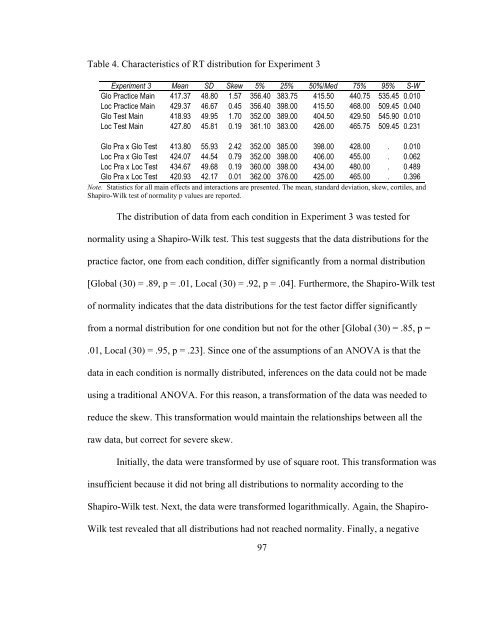
Table 4. Characteristics of RT distribution for Experiment 3 Experiment 3 Mean SD Skew 5% 25% 50%/Med 75% 95% S-W Glo Practice Main 417.37 48.80 1.57 356.40 383.75 415.50 440.75 535.45 0.010 Loc Practice Main 429.37 46.67 0.45 356.40 398.00 415.50 468.00 509.45 0.040 Glo Test Main 418.93 49.95 1.70 352.00 389.00 404.50 429.50 545.90 0.010 Loc Test Main 427.80 45.81 0.19 361.10 383.00 426.00 465.75 509.45 0.231 Glo Pra x Glo Test 413.80 55.93 2.42 352.00 385.00 398.00 428.00 . 0.010 Loc Pra x Glo Test 424.07 44.54 0.79 352.00 398.00 406.00 455.00 . 0.062 Loc Pra x Loc Test 434.67 49.68 0.19 360.00 398.00 434.00 480.00 . 0.489 Glo Pra x Loc Test 420.93 42.17 0.01 362.00 376.00 425.00 465.00 . 0.396 Note. Statistics for all main effects and interactions are presented. The mean, standard deviation, skew, cortiles, and Shapiro-Wilk test of normality p values are reported. The distribution of data from each condition in Experiment 3 was tested for normality using a Shapiro-Wilk test. This test suggests that the data distributions for the practice factor, one from each condition, differ significantly from a normal distribution [Global (30) = .89, p = .01, Local (30) = .92, p = .04]. Furthermore, the Shapiro-Wilk test of normality indicates that the data distributions for the test factor differ significantly from a normal distribution for one condition but not for the other [Global (30) = .85, p = .01, Local (30) = .95, p = .23]. Since one of the assumptions of an ANOVA is that the data in each condition is normally distributed, inferences on the data could not be made using a traditional ANOVA. For this reason, a transformation of the data was needed to reduce the skew. This transformation would maintain the relationships between all the raw data, but correct for severe skew. Initially, the data were transformed by use of square root. This transformation was insufficient because it did not bring all distributions to normality according to the Shapiro-Wilk test. Next, the data were transformed logarithmically. Again, the Shapiro- Wilk test revealed that all distributions had not reached normality. Finally, a negative 97
Page 1 and 2:
Time Course of Perceptual Grouping
Page 3 and 4:
Experiment 1 76 Method 76 Results a
Page 5 and 6:
List of Figures Figure 1. Illustrat
Page 7 and 8:
Page 9 and 10:
Page 11 and 12:
will look like and how it will comm
Page 13 and 14:
visibility of important interface e
Page 15 and 16:
displays are reported. Global and l
Page 17 and 18:
Electrical activity generated by th
Page 19 and 20:
would not be. It would be easier to
Page 21 and 22:
could be grouped by the principles
Page 23 and 24:
Figure 4. Gestalt principles of gro
Page 25 and 26:
One of the leaders in grouping and
Page 27 and 28:
defined by similar numbers. For exa
Page 29 and 30:
and Saasrinen (2000) observed that
Page 31 and 32:
proximity (Bailey, 1989; Bonney & W
Page 33 and 34:
find the target ‘Picture’ in th
Page 35 and 36:
Humans integrate many types of info
Page 37 and 38:
measures. As a result, the pilot wo
Page 39 and 40:
Figure 10. Pop-up advertisement wit
Page 41 and 42:
soldiers see in these speeded condi
Page 43 and 44:
2001), grouping by proximity and al
Page 45 and 46:
local letters, as illustrated by Fi
Page 47 and 48:
frequency channels at specific rang
Page 49 and 50:
Recent support for the Flexible Usa
Page 51 and 52:
occluded shape as being incomplete
Page 53 and 54: search for the target in the experi
Page 55 and 56: Gestalt principle of good continuat
Page 57 and 58: columns of circles on the opposing
Page 59 and 60: short stimulus durations can be use
Page 61 and 62: Figure 15. Results for ambiguous pr
Page 63 and 64: As shown in Figure 16B, for the lig
Page 65 and 66: In review these findings, it become
Page 67 and 68: in user interface display layouts.
Page 69 and 70: were asked to make decisions about
Page 71 and 72: columns of pushbuttons on either si
Page 73 and 74: principles that are depicted more g
Page 75 and 76: no longer perceived. These cases wi
Page 77 and 78: influence what ‘goes together’
Page 79 and 80: participants, randomly with replace
Page 81 and 82: Figure 23. Targets used in reported
Page 83 and 84: participants that were more than th
Page 85 and 86: that was presented in the pilot exp
Page 87 and 88: from three participants because one
Page 89 and 90: see, each of the four distributions
Page 91 and 92: The distribution of data from each
Page 93 and 94: Figure 28. Targets for Experiment 2
Page 95 and 96: Results and discussion Sixteen fema
Page 97 and 98: global grouping was significantly f
Page 99 and 100: Figure 32A depicts a box plot for g
Page 101 and 102: means, the Wilcoxon Signed Ranks Te
Page 103: to group by the alternative scale.
Page 107 and 108: General Discussion Research that ha
Page 109 and 110: Experiments 2A and 2B were designed
Page 111 and 112: the size scale within an existing i
Page 113 and 114: “Hotmail” has been reported to
Page 115 and 116: They are interesting within the con
Page 117 and 118: forms of similarity could also be t
Page 119 and 120: the context of vision science resea
Page 121 and 122: Bennett, K. B., Nagy, A. L., and Fl
Page 123 and 124: De Valois, R. L. & De Valois, K. K.
Page 125 and 126: Johnston, W.A., Schwarting, I.S. &
Page 127 and 128: Nass, C., Isbister, K., & Lee, E.J.
Page 129 and 130: Palmer, S. E. & Rock, I. (1994). Re
Page 131 and 132: Sanocki, T.(2001). Interaction of s
Page 133 and 134: Tullis, T. S. (1981). An evaluation
Page 135: About the Author Melissa F. Schulz
show all

The Use of Iambic Pentameter in the

Create successful ePaper yourself

Delete template?

Save as template?