a la physique de l'information - Lisa - Université d'Angers

It is assumed that the signal s is weak, so that σ 2 s ≪ 1.
The linear minimum mean square error estimator ˆs of
the signal s is given by the well known Wiener £lter [1]
ˆs = CsxC −1
xxx , (4)
where Cxx is the covariance matrix of x and Csx is the
cross-covariance matrix of s and x. As Csx = Css and
Cxx = Css + Cηη with Cηη = I, the estimated signal ˆs
is given by
ˆs = Css(Css + I) −1 x . (5)
Using the weak signal approximation, σ 2 s ≪ 1, we get
ˆs = Cssx . (6)
When the additive noise η is Gaussian the linear Wiener
Filter turns out to be the overall (among all linear or nonlinear
classes) optimal estimator minimizing the mean square
error of the estimated signal ˆs with respect to the original
signal s. But, as soon as one departs from the case of a
Gaussian noisy environment, the optimality of the Wiener
£lter is no longer assured. Still, because of its simplicity of
implementation, due to its linear property, the Wiener £lter
is often used even in the presence of non-Gaussian noise.
However, the performance of the Wiener £lter in such non-
Gaussian noisy conditions can be quite poor.
For our estimation task, we will speci£cally consider
η to be non-Gaussian noise. For illustration, we examine
two noise famillies: generalized Gaussian noise, and mixture
of Gaussian noise.The pdf of the generalized Gaussian
noise is expressed as fη(u) = fgg(u/ση)/ση, using the
standardized density
fgg(u) = A exp(− | bu | p ) , (7)
where σ 2 η is the variance, b = [Γ(3/p)/Γ(1/p)] 1/2 and A =
(p/2)[Γ(3/p)] 1/2 /[Γ(1/p)] 3/2 are parameterized by the positive
exponent p. This family is interesting in the present
situation for it includes the Gaussian case (p = 2). Furthermore,
generalized Gaussian densities enable one to study
noise whose tails are either heavier (p < 2) or lighter (p >
2) than that of the Gaussian noise. The mixture of Gaussian
pdf is expressed as fη(u) = fmg(u/ση)/ση, using the
standardized density
fmg(u) =
c
√ α exp −
2π
c2u2
2
+ 1 − α
exp −
β
c2u2 2β2 , (8)
where c = [α + (1 − α)(β 2 )] 1/2 ; σ 2 η is the variance, α ∈
[0, 1] is the mixing parameter and β > 0 is the ratio of
the standard deviations of the individual contributions. This
family of pdf’s is a subclass of Middleton’s class wich is
also widely used to model ocean acoustic noise [2]. In the
next section, we introduce a simple nonlinear estimator and
compare its performance with that of the Wiener £lter in
the presence of generalized Gaussian or mixture of Gaussian
noise.
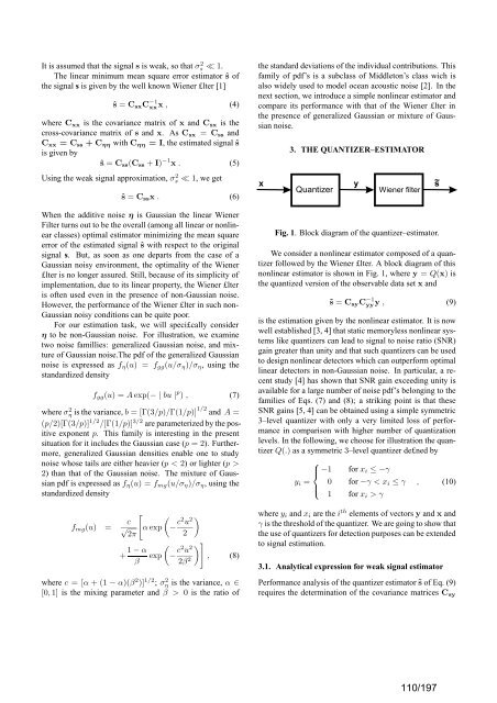
3. THE QUANTIZER–ESTIMATOR
Fig. 1. Block diagram of the quantizer–estimator.
We consider a nonlinear estimator composed of a quantizer
followed by the Wiener £lter. A block diagram of this
nonlinear estimator is shown in Fig. 1, where y = Q(x) is
the quantized version of the observable data set x and
˜s = CsyC −1
yyy , (9)
is the estimation given by the nonlinear estimator. It is now
well established [3, 4] that static memoryless nonlinear systems
like quantizers can lead to signal to noise ratio (SNR)
gain greater than unity and that such quantizers can be used
to design nonlinear detectors which can outperform optimal
linear detectors in non-Gaussian noise. In particular, a recent
study [4] has shown that SNR gain exceeding unity is
available for a large number of noise pdf’s belonging to the
families of Eqs. (7) and (8); a striking point is that these
SNR gains [5, 4] can be obtained using a simple symmetric
3–level quantizer with only a very limited loss of performance
in comparison with higher number of quantization
levels. In the following, we choose for illustration the quantizer
Q(.) as a symmetric 3–level quantizer de£ned by
⎧
⎪⎨ −1 for xi ≤ −γ
yi = 0 for −γ < xi ≤ γ , (10)
⎪⎩
1 for xi > γ
where yi and xi are the i th elements of vectors y and x and
γ is the threshold of the quantizer. We are going to show that
the use of quantizers for detection purposes can be extended
to signal estimation.
3.1. Analytical expression for weak signal estimator
Performance analysis of the quantizer estimator ˜s of Eq. (9)
requires the determination of the covariance matrices Csy
110/197