a la physique de l'information - Lisa - Université d'Angers

Author's personal copy
3982 F. Chapeau-Blondeau, D. Rousseau / Physica A 388 (2009) 3969–3984
each axis, leading to a total number K = K D
0 of cells in D dimensions. The search for the minimization of Ltotal is then now
reduced to a one-dimensional search in K0. A much simpler minimization process results, at the price of reduced resolution
in the D-dimensional histograms. Other strategies can be envisaged to organize the division of the coordinate axes associated
with the MDL criterion. In this same direction of multidimensional histograms with MDL, a recent study [41] introduces a
new family of multidimensional histograms in the context of data mining for query answering. A local parametric model is
employed to describe each multidimensional bin of the histogram, and local application of MDL is performed to optimize
the parameterization. This approach of Ref. [41] is reminiscent of kernel methods, which form a different methodology
for probability density estimation based on a definite choice of parametric kernel functions, and which although quite
distinct from histograms, can also be handled with MDL for optimal parameterization. Beyond histogram estimation, such
extensions of the MDL principle naturally offer, as suggested by the examples of Fig. 7, flexible and optimal subquantizations
of multidimensional data based on an informational principle. This can be very useful for reduction of the complexity of
multidimensional data sets, which are more and more pervasive in many areas of observational sciences, and with a control
of the procedure obtained in an informational framework.
Appendix. Quantization of continuously-valued parameters
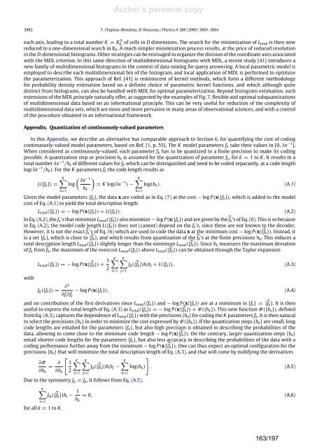
In this Appendix, we describe an alternative but comparable approach to Section 6, for quantifying the cost of coding
continuously-valued model parameters, based on Ref. [1, p. 55]. The K model parameters fk take their values in [0, δx −1 ].
When considered as continuously-valued, each parameter fk has to be quantized to a finite precision to make its coding
possible. A quantization step or precision hk is assumed for the quantization of parameter fk, for k = 1 to K . It results in a
total number δx −1 /hk of different values for fk which can be distinguished and need to be coded separately, at a code length
log(δx −1 /hk). For the K parameters fk the code length results as
K
−1
δx
L({fk}) = log = K log(δx −1 K
) − log(hk). (A.1)
k=1
hk
k=1
Given the model parameters {fk}, the data x are coded as in Eq. (7) at the cost − log P(x|{fk}), which is added to the model
cost of Eq. (A.1) to yield the total description length
Ltotal({fk}) = − log P(x|{fk}) + L({fk}). (A.2)
In Eq. (A.2), the fk’s that minimize Ltotal({fk}) also minimize − log P(x|{fk}) and are given by the fk’s of Eq. (6). This is so because
in Eq. (A.2), the model code length L({fk}) does not (cannot) depend on the fk’s, since these are not known to the decoder.
However, it is not the exact fk’s of Eq. (6) which are used to code the data x at the minimum cost − log P(x|{ fk}). Instead, it
is a set {fk}, which is close to { fk}, and which results from quantization of the fk’s at the finite precisions hk. This induces a
total description length Ltotal({fk}) slightly longer than the minimum Ltotal({ fk}). Since hk measures the maximum deviation
of fk from fk, the maximum of the overcost Ltotal({fk}) above Ltotal({ fk}) can be obtained through the Taylor expansion
with
Ltotal({fk}) = − log P(x|{ fk}) + 1
Jij({fk}) =
∂ 2
∂fi∂fj
2
K
i=1
K
Jij({fk})hihj + L({fk}), (A.3)
j=1
− log P(x|{fk}), (A.4)
and no contribution of the first derivatives since Ltotal({fk}) and − log P(x|{fk}) are at a minimum in {fk} = {fk}. It is then
useful to express the total length of Eq. (A.3) as Ltotal({fk}) = − log P(x|{fk}) + Φ({hk}). This new function Φ({hk}), defined
from Eq. (A.3), captures the dependence of Ltotal({fk}) with the precisions {hk} for coding the K parameters fk. It is then natural
to select the precisions {hk} in order to minimize the cost expressed by Φ({hk}). If the quantization steps {hk} are small, long
code lengths are entailed for the parameters {fk}, but also high precision is obtained in describing the probabilities of the
data, allowing to come close to the minimum code length − log P(x|{fk}). On the contrary, larger quantization steps {hk}
entail shorter code lengths for the parameters {fk}, but also less accuracy in describing the probabilities of the data with a
coding performance further away from the minimum − log P(x|{fk}). One can thus expect an optimal configuration for the
precisions {hk} that will minimize the total description length of Eq. (A.3), and that will come by nullifying the derivatives
∂Φ
= ∂
K K
K
1
Jij({fk})hihj − log(hk) . (A.5)
2
∂hk
∂hk
i=1
j=1
k=1
Due to the symmetry Jij = Jji, it follows from Eq. (A.5),
K
Jik({fk})hi − 1
= 0, (A.6)
i=1
for all k = 1 to K .
hk
163/197