a la physique de l'information - Lisa - Université d'Angers

probability of error (expected as small as possible).
This Bayesian detection strategy requires that
probabilities (P0, P1 ¼ 1 P0) of both hypotheses
(respectively, H0, H1) of Eq. (2) are known. This
assumption, typically valid in the domain of
telecommunication, is not possible in other applications
such as sonar or radar [2]. When P0 and P1 are
unknown, if the decision between (hypothesis H1)
and (hypothesis H0) is directly based on the linear
signal–noise mixture, the observable data set x, a
strategy to implement an optimal detection is to
seek to maximize the probability of detection
Z
PD ¼ pðxjH1Þ dx, (21)
R1
while keeping the probability of false alarm
Z
PF ¼ pðxjH0Þ dx (22)
R1
no larger than a prescribed level PF;sup. This
constrained maximization is achieved by the optimal
Neyman–Pearson detector, which also implements
a likelihood-ratio test. When the input noise
xðtÞ is Gaussian the best detector in the Neyman–
Pearson sense takes a form very similar to the linear
detector described in Fig. 1a [2]: a correlation
receiver which computes the statistic TðxÞ ¼
P N 1
j¼0 xðtjÞsðtjÞ is followed by the Neyman–Pearson
likelihood-ratio test based on this statistic TðxÞ,
LðTðxÞÞ _ H1
mðPF;supÞ, (23)
H0
with a threshold mðPF;supÞ, a function of PF;sup,
which is found from Eq. (22) by imposing
PFpPF;sup. The probability of detection of this
Neyman–Pearson linear detector is given by
PD ¼ erfc erfc 1 ðPF;supÞ s0
s1
m1 m0
s0
(24)
with, for k 2f0; 1g, means mk ¼ E½TðxÞjHkŠ,
variance s2 k ¼ var½TðxÞjHkŠ and erfcðuÞ ¼ R þ1
u ð1=
pffiffiffiffiffi 2 2pÞ
expð v =2Þ dv. When the input noise xðtÞ is
non-Gaussian, the optimal detector in the Neyman–
Pearson, in general, is difficult to design. The same
nonlinear array of Fig. 2 can be used again as
preprocessor to design a simple suboptimal nonlinear
detector capable of outperforming the
Neyman–Pearson linear detector when the input
noise xðtÞ is non-Gaussian. Therefore, this
Neyman–Pearson nonlinear detector first applies
the observable data set x ¼ðxðt1Þ; ...; xðtNÞÞ at the
ARTICLE IN PRESS
D. Rousseau et al. / Signal Processing 86 (2006) 3456–3465 3463
probability of detection P D
0.7
0.6
0.5
0.4
0.3
0.2
0 0.5 1 1.5 2 2.5 3
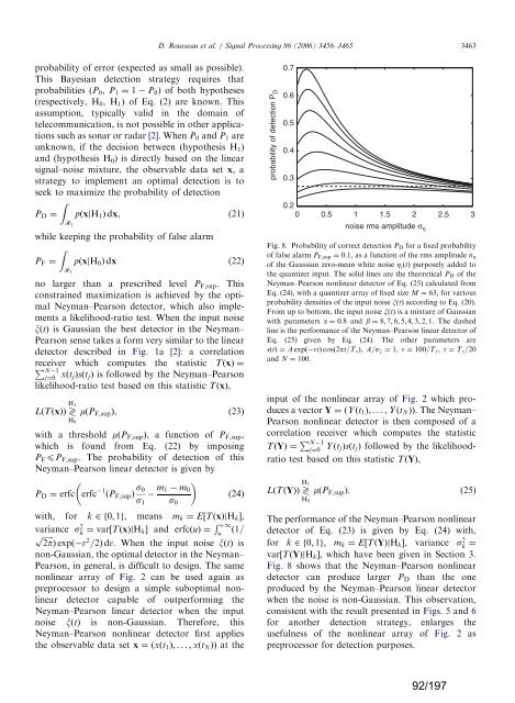
noise rms amplitude ση Fig. 8. Probability of correct detection PD for a fixed probability
of false alarm PF;sup ¼ 0:1, as a function of the rms amplitude sZ
of the Gaussian zero-mean white noise Z iðtÞ purposely added to
the quantizer input. The solid lines are the theoretical PD of the
Neyman–Pearson nonlinear detector of Eq. (25) calculated from
Eq. (24), with a quantizer array of fixed size M ¼ 63, for various
probability densities of the input noise xðtÞ according to Eq. (20).
From up to bottom, the input noise xðtÞ is a mixture of Gaussian
with parameters a ¼ 0:8 and b ¼ 8; 7; 6; 5; 4; 3; 2; 1. The dashed
line is the performance of the Neyman–Pearson linear detector of
Eq. (25) given by Eq. (24). The other parameters are
sðtÞ ¼A expð ntÞ cosð2pt=T sÞ, A=sx ¼ 1, n ¼ 100=T s, t ¼ T s=20
and N ¼ 100.
input of the nonlinear array of Fig. 2 which produces
a vector Y ¼ðYðt1Þ; ...; YðtNÞÞ. The Neyman–
Pearson nonlinear detector is then composed of a
correlation receiver which computes the statistic
TðYÞ ¼ PN 1
j¼0 YðtjÞsðtjÞ followed by the likelihoodratio
test based on this statistic TðYÞ,
LðTðYÞÞ _ H1
mðPF;supÞ. (25)
H0
The performance of the Neyman–Pearson nonlinear
detector of Eq. (23) is given by Eq. (24) with,
for k 2f0; 1g, mk ¼ E½TðYÞjHkŠ, variance s 2 k ¼
var½TðYÞjHkŠ, which have been given in Section 3.
Fig. 8 shows that the Neyman–Pearson nonlinear
detector can produce larger PD than the one
produced by the Neyman–Pearson linear detector
when the noise is non-Gaussian. This observation,
consistent with the result presented in Figs. 5 and 6
for another detection strategy, enlarges the
usefulness of the nonlinear array of Fig. 2 as
preprocessor for detection purposes.
92/197