a la physique de l'information - Lisa - Université d'Angers

2660 IEEE TRANSACTIONS ON INSTRUMENTATION AND MEASUREMENT, VOL. 56, NO. 6, DECEMBER 2007
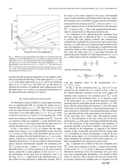
Fig. 1. RMS error of the optimal Bayesian estimator as a function of the rms
amplitude ση of the threshold noises ηi(t) chosen zero-mean Gaussian. The
input noise ξ(t) is a zero-mean Gaussian with an rms amplitude σξ =1.The
prior pdf pa(u) is a zero-mean Gaussian with an rms amplitude σa =1.All
the thresholds in the array are set to θ =0, with M =1. The solid lines are
E 1/2
B from the theory of (8). The dashed line is the estimation error σBin from
(13) of the same optimal (minimal error) estimator operating directly on the
input-signal–noise mixture xa(t).
possibly through numerical integration, for any definite conditions
concerning the following: 1) the input signal via sa(t) and
pa(u); 2) the input white noise via fξ(u), and 3) the measuring
array via θ, N, and Fη(u). We shall now use this theory to
illustrate the existence of conditions where enhancement of the
threshold noises ηi(t) results in an improved performance for
the optimal Bayesian estimator of a from Y .
III. NOISE-IMPROVED ESTIMATION
For illustration of the possibility of a noise-improved estimation
via suprathreshold SR, we consider the simple case of a
constant input signal sa(t) ≡ a. The input noise ξ(t) is taken
with zero mean and rms amplitude σξ. The common threshold
in the array is set at the input mean, i.e., θ = E[xa(t)], which
is known as soon as pa(u) and fξ(u) are specified. Fig. 1 then
shows the evolution of the rms estimation error E 1/2
B from (8)
as a function of the rms amplitude ση of the threshold noises
for various sizes N of the array when both the input noise ξ(t)
and the threshold noises ηi(t) are zero-mean Gaussian.
In Fig. 1, the choice θ = E[xa(t)] ensures that the inputsignal–noise
mixture xa(t) is suprathreshold, in the sense that
xa(t) evolves on both sides of the threshold θ and can cross θ
without assistance from the threshold noises ηi(t). As a consequence,
if the array is reduced to a single device (N =1),the
added threshold noise η1(t) does not improve the performance,
and its increase monotonically degrades the estimation error
E 1/2
B , as shown in Fig. 1. When N>1, in the absence of the
threshold noises ηi(t), all the quantizers in the array switch in
unison, acting like a single quantizer. In this case, at ση =0,
the performance of the array does not depend on size N of
the array. At N>1, application of the threshold noises ηi(t)
then allows for the quantizers to differently respond. This is
the source of the richer response of the array with threshold
noises. For the estimation task performed from the array output,
this translates into a possibility of improving the performance
measured by the estimation error E 1/2
B , with, for each N>1,a
nonzero optimal amount of the threshold noises that minimizes
E 1/2
B , as shown in Fig. 1. This is the suprathreshold SR effect,
which is reported here in a Bayesian estimation task.
For comparison of the optimal Bayesian estimation from
the array output that is addressed in Fig. 1, it is interesting
to consider the same optimal estimator (the minimal-error
estimator) that would directly operate on the input-signal–noise
mixture xa(t) rather than on its quantized representation by the
array. By applying on xa(t) the principles of optimal Bayesian
estimation similar to those exposed in Section II, it comes out
that, when the input noise ξ(t) is zero-mean Gaussian, the
optimal Bayesian estimator [31] operating directly on xa(t) is
aBin, which achieves the rms estimation error σBin, verifying
1
σ 2 Bin
with the estimator itself reading
aBin = σ2 Bin
σ 2 a
= 1
σ2 +
a
M
σ2 ξ
E(a)+M σ2 Bin
σ2 xa
ξ
(13)
(14)
with the empirical mean of the measurements xa =
M −1 M
j=1 xa(tj).
In Fig. 1, the rms estimation error σBin from (13) is represented
by the dashed line. It is shown in Fig. 1 that, in
the optimal Bayesian estimation from the array output, the
minimal value reached by the estimation error E 1/2
B
at the
optimal level of the threshold noises, as N increases, tends
to the performance σBin of the optimal Bayesian estimator
operating directly on the input-signal–noise mixture xa(t).This
proves that the optimal Bayesian estimator aB from the output
of the array of one-bit quantizers, as the array becomes large, is
able to perform as efficiently as the optimal Bayesian estimator
aBin operating directly on the input-signal–noise mixture xa(t).
At the same time, Fig. 1 shows that, with relatively modest
sizes N, the performance of the array comes close to the best
performance σBin at the input. Advantages afforded by the array
lie in the parsimony of the representation and simplicity of
operation (possibly associated to rapidity), working on a few
bits collected by the comparators, as opposed to the infinite
number of bits, in principle, associated with the analog input
xa(t). In addition, in various circumstances, it may be the case
that the analog input xa(t) is not directly accessible when no
linear transducers are available to form a direct image of xa(t)
that is manageable by the signal-processing system.
Fig. 2 represents the evolution of the rms estimation error
E 1/2
B in the same conditions as in Fig. 1, except for the number
of data points M =2. As usual, in Bayesian estimation, the
theoretical calculation of the rms estimation error gets more
and more computationally demanding as the number of data
points M increases. This is because the rms error results from
an average (expressed by multiple sums or integrals) over all
81/197