a la physique de l'information - Lisa - Université d'Angers

Author's personal copy
3978 F. Chapeau-Blondeau, D. Rousseau / Physica A 388 (2009) 3969–3984
A B
total description length
x 10 6
1.5172
1.5171
1.517
1.5169
1.5168
1.5167
1.5166
1.5165
1.5164
0 10 20 30 40 50 60 70 80 100 120 150 170
number of bins K
3
2
4
probability density
0.4
0.3
0.2
0.1
0
–4 –3 –2 –1 0 1 2 3 4 5 6
signal amplitude
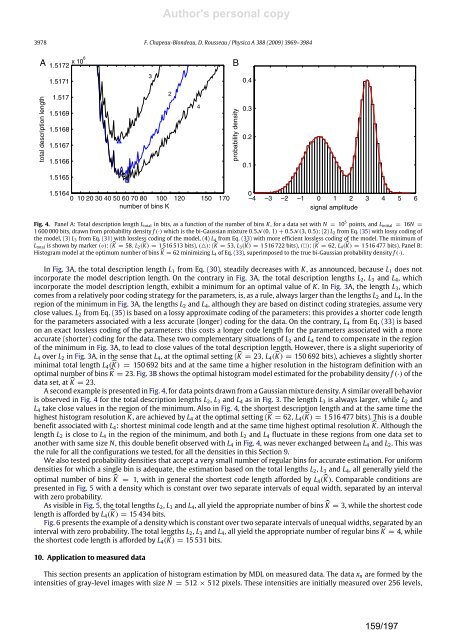
Fig. 4. Panel A: Total description length Ltotal in bits, as a function of the number of bins K , for a data set with N = 10 5 points, and Linitial = 16N =
1 600 000 bits, drawn from probability density f (·) which is the bi-Gaussian mixture 0.5N (0, 1) + 0.5N (3, 0.5): (2) L2 from Eq. (35) with lossy coding of
the model, (3) L3 from Eq. (31) with lossless coding of the model, (4) L4 from Eq. (33) with more efficient lossless coding of the model. The minimum of
Ltotal is shown by marker (◦): ( K = 58, L2( K) = 1 516 513 bits), (△): ( K = 53, L3( K) = 1 516 722 bits), (): ( K = 62, L4( K) = 1 516 477 bits). Panel B:
Histogram model at the optimum number of bins K = 62 minimizing L4 of Eq. (33), superimposed to the true bi-Gaussian probability density f (·).
In Fig. 3A, the total description length L1 from Eq. (30), steadily decreases with K , as announced, because L1 does not
incorporate the model description length. On the contrary in Fig. 3A, the total description lengths L2, L3 and L4, which
incorporate the model description length, exhibit a minimum for an optimal value of K . In Fig. 3A, the length L3, which
comes from a relatively poor coding strategy for the parameters, is, as a rule, always larger than the lengths L2 and L4. In the
region of the minimum in Fig. 3A, the lengths L2 and L4, although they are based on distinct coding strategies, assume very
close values. L2 from Eq. (35) is based on a lossy approximate coding of the parameters: this provides a shorter code length
for the parameters associated with a less accurate (longer) coding for the data. On the contrary, L4 from Eq. (33) is based
on an exact lossless coding of the parameters: this costs a longer code length for the parameters associated with a more
accurate (shorter) coding for the data. These two complementary situations of L2 and L4 tend to compensate in the region
of the minimum in Fig. 3A, to lead to close values of the total description length. However, there is a slight superiority of
L4 over L2 in Fig. 3A, in the sense that L4, at the optimal setting ( K = 23, L4( K) = 150 692 bits), achieves a slightly shorter
minimal total length L4( K) = 150 692 bits and at the same time a higher resolution in the histogram definition with an
optimal number of bins K = 23. Fig. 3B shows the optimal histogram model estimated for the probability density f (·) of the
data set, at K = 23.
A second example is presented in Fig. 4, for data points drawn from a Gaussian mixture density. A similar overall behavior
is observed in Fig. 4 for the total description lengths L2, L3 and L4 as in Fig. 3. The length L3 is always larger, while L2 and
L4 take close values in the region of the minimum. Also in Fig. 4, the shortest description length and at the same time the
highest histogram resolution K , are achieved by L4 at the optimal setting ( K = 62, L4( K) = 1 516 477 bits). This is a double
benefit associated with L4: shortest minimal code length and at the same time highest optimal resolution K . Although the
length L2 is close to L4 in the region of the minimum, and both L2 and L4 fluctuate in these regions from one data set to
another with same size N, this double benefit observed with L4 in Fig. 4, was never exchanged between L4 and L2. This was
the rule for all the configurations we tested, for all the densities in this Section 9.
We also tested probability densities that accept a very small number of regular bins for accurate estimation. For uniform
densities for which a single bin is adequate, the estimation based on the total lengths L2, L3 and L4, all generally yield the
optimal number of bins K = 1, with in general the shortest code length afforded by L4( K). Comparable conditions are
presented in Fig. 5 with a density which is constant over two separate intervals of equal width, separated by an interval
with zero probability.
As visible in Fig. 5, the total lengths L2, L3 and L4, all yield the appropriate number of bins K = 3, while the shortest code
length is afforded by L4( K) = 15 434 bits.
Fig. 6 presents the example of a density which is constant over two separate intervals of unequal widths, separated by an
interval with zero probability. The total lengths L2, L3 and L4, all yield the appropriate number of regular bins K = 4, while
the shortest code length is afforded by L4( K) = 15 531 bits.
10. Application to measured data
This section presents an application of histogram estimation by MDL on measured data. The data xn are formed by the
intensities of gray-level images with size N = 512 × 512 pixels. These intensities are initially measured over 256 levels,
159/197