software to fit optical spectra - Quantum Materials Group

Equation 2-6
N 1 ∂f
∂f
α kl
( x , 1,
, ) ( , 1,
, )
2
i p K pM
xi
p K pM
.
∂p
∂p
≡ ∑
i= 1 σ i
k
l
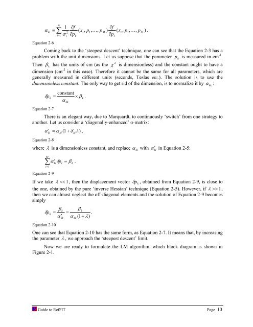
Coming back to the ‘steepest descent’ technique, one can see that the Equation 2-3 has a
problem with the unit dimensions. Let us suppose that the parameter p k is measured in cm -1 .
Then β k has the units of cm (as the
2
χ is dimensionless) and the constant ought to have a
dimension (cm -2 in this case). Therefore it cannot be the same for all parameters, which are
generally measured in different units (seconds, Teslas etc.). The solution is to use the
dimensionless constant. The only way to get rid of the dimension, is to normalize it by α kk :
Equation 2-7
constant
δ p k = × β k .
α
kk
There is an elegant way, due to Marquardt, to continuously ‘switch’ from one strategy to
another. Let us consider a ‘diagonally-enhanced’ α-matrix:
′ = α ( 1+
δ λ)
,
Equation 2-8
α kl kl kl
where λ is a dimensionless constant, and replace α kl with α ′ kl in Equation 2-5:
M
∑
i=
1
Equation 2-9
α ′ δ = β .
kl pl
k
If we take λ > 1,
then we can almost neglect the off-diagonal elements and the solution of Equation 2-9 becomes
simply
β k β k
δp
k = = .
α ′ α ( 1+
λ)
Equation 2-10
kk
kk
One can see that Equation 2-10 has the same form, as Equation 2-7. It means that, by increasing
the parameter λ , we approach the ‘steepest descent’ limit.
Now we are ready to formulate the LM algorithm, which block diagram is shown in
Figure 2-1.
Guide to RefFIT Page 10