software to fit optical spectra - Quantum Materials Group

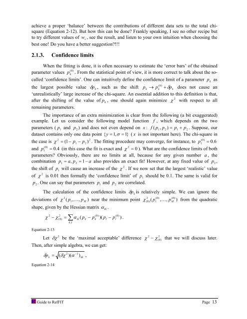
achieve a proper ‘balance’ between the contributions of different data sets to the total chisquare
(Equation 2-12). But how this can be done? Frankly speaking, I see no other recipe but
to try different values of w v , see the result, and listen to your own intuition when choosing the
best one! Do you have a better suggestion?!!!
2.1.3. Confidence limits
When the fitting is done, it is often necessary to estimate the ‘error bars’ of the obtained
( 0)
parameter values p k . From the statistical point of view, it is more correct to talk about the socalled
‘confidence limits’. One can intuitively define the confidence limit of a parameter p k as
the largest possible value δ pk
, such as the shift pk → pk
+ δpk
) 0 (
does not cause an
‘unrealistically’ large increase of the chi-square. An essential addition to this definition is that,
after the shifting of the value of p k , one should again minimize 2
χ with respect to all
remaining parameters.
The importance of an extra minimization is clear from the following (a bit exaggerated)
example. Let us consider the following model function f , which depends on the two
parameters ( 1 p and 2 p ) and does not even depend on x : f ( p1
, p2
) = p1
+ p2
. Suppose, our
dataset contains only one data point { y = 1,
σ = 1}
( x is not important here). The chi-square in
2
2
( 0)
the case is χ = ( 1−
p1 − p2
) . The fitting procedure may converge, for instance, to p 1 = 0.
6
( 0)
2
and p 1 = 0.
4 (in this case the fit is exact and χ = 0 ). What are the confidence limits of both
parameters? Obviously, there are no limits at all, because for any given number a , the
combination p1 = a,
p2
= 1−
a also provides an exact fit! However, at any fixed value of p 2 ,
2
the shift of p 1 will cause an increase of the χ . If we now set that the largest ‘realistic’ value
2
of χ is 0.01 then formally the ‘confidence limit’ of p 1 should be 0.1. The same is valid for
p are correlated.
p 2 . One can say that parameters 1 p and 2
The calculation of the confidence limits δpk is relatively simple. We can ignore the
2
2 ( 0)
( 0)
deviations of χ ( p1, K,
pM
) near the minimum point χ ( 0)
( p1 , K,
pM
) from the quadratic
shape, given by the Hessian matrix α kl .
2 2
( 0)
( 0)
χ − χ ( 0)
= ∑α kl ( pk
− pk
)( pl
− pl
) .
Equation 2-13
k , l
Let
Then, after simple algebra, we can get:
k
2
δχ be the ‘maximal acceptable’ difference
2 −1
δ p = ( δχ )( α ) ,
Equation 2-14
kk
2 2
χ − χ ( 0)
that we will discuss later.
Guide to RefFIT Page 13