software to fit optical spectra - Quantum Materials Group

More documents

Recommendations

Info

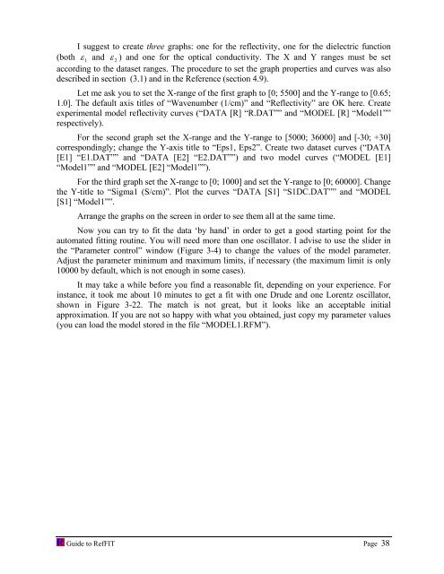
I suggest to create three graphs: one for the reflectivity, one for the dielectric function (both ε 1 and ε 2 ) and one for the optical conductivity. The X and Y ranges must be set according to the dataset ranges. The procedure to set the graph properties and curves was also described in section (3.1) and in the Reference (section 4.9). Let me ask you to set the X-range of the first graph to [0; 5500] and the Y-range to [0.65; 1.0]. The default axis titles of “Wavenumber (1/cm)” and “Reflectivity” are OK here. Create experimental model reflectivity curves (“DATA [R] “R.DAT”” and “MODEL [R] “Model1”” respectively). For the second graph set the X-range and the Y-range to [5000; 36000] and [-30; +30] correspondingly; change the Y-axis title to “Eps1, Eps2”. Create two dataset curves (“DATA [E1] “E1.DAT”” and “DATA [E2] “E2.DAT””) and two model curves (“MODEL [E1] “Model1”” and “MODEL [E2] “Model1””). For the third graph set the X-range to [0; 1000] and set the Y-range to [0; 60000]. Change the Y-title to “Sigma1 (S/cm)”. Plot the curves “DATA [S1] “S1DC.DAT”” and “MODEL [S1] “Model1””. Arrange the graphs on the screen in order to see them all at the same time. Now you can try to fit the data ‘by hand’ in order to get a good starting point for the automated fitting routine. You will need more than one oscillator. I advise to use the slider in the “Parameter control” window (Figure 3-4) to change the values of the model parameter. Adjust the parameter minimum and maximum limits, if necessary (the maximum limit is only 10000 by default, which is not enough in some cases). It may take a while before you find a reasonable fit, depending on your experience. For instance, it took me about 10 minutes to get a fit with one Drude and one Lorentz oscillator, shown in Figure 3-22. The match is not great, but it looks like an acceptable initial approximation. If you are not so happy with what you obtained, just copy my parameter values (you can load the model stored in the file “MODEL1.RFM”). Guide to RefFIT Page 38
Figure 3-22 The general RefFIT view after the data fitting ‘by hand’. OK, it is time for computer to work a little bit and refine the model parameters. We only have to set up the fitting task to tell him what exactly we want to fit. Open the “Fit” window (Figure 3-12). We have to specify the chi-square terms 2 χ ν and their weights ν w from Equation 2-12. Click the button. In the window “Add Chi-square term(s)” (Figure 3-23) select all available terms: “[S1] “S1DC.DAT” – “Model1””, “[E2] “E2.DAT” – “Model1””, “[E1] “E1.DAT” – “Model1”” and “[R] “R.DAT” – “Model1”” and click . Guide to RefFIT Page 39
Page 1 and 2: Last updated: 20.04.2004 Guide to R
Page 3 and 4: 4.8. Dataset manager ..............
Page 5 and 6: that time. The later development of
Page 7 and 8: 1.4. Let’s keep in touch Please,
Page 9 and 10: 2.1.1. Levenberg-Marquardt algorith
Page 11 and 12: Guess initial parameters p , , p 1
Page 13 and 14: achieve a proper ‘balance’ betw
Page 15 and 16: The third requirement is that at ve
Page 17 and 18: Equation 2-19 is useful to estimate
Page 19 and 20: The first problem is that the Loren
Page 21 and 22: The problem can be circumvented by
Page 23 and 24: In these cases the fitting of the d
Page 25 and 26: 3. Tutorial This chapter shows how
Page 27 and 28: Figure 3-3 Graph contents window is
Page 29 and 30: Figure 3-7 Click the button and in
Page 31 and 32: If you are still far from this fitt
Page 33 and 34: Figure 3-15 The model and experimen
Page 35 and 36: Figure 3-18 The “Graph properties
Page 37: Figure 3-20 Loading the reflectivit
Page 41 and 42: Figure 3-25 The general RefFIT view
Page 43 and 44: MainWindow(XPos = 0, YPos = 0, Widt
Page 45 and 46: emarkable ‘anomaly’, related to
Page 47 and 48: ###################################
Page 49 and 50: # restores the original application
Page 51 and 52: 4. Reference 4.1. System requiremen
Page 53 and 54: Figure 4-2 The “Parameter control
Page 55 and 56: The model file stores information a
Page 57 and 58: considering multiple (Fabri- Perot)
Page 59 and 60: optical conductivity in practical u
Page 61 and 62: Kronig friendly, so be careful! “
Page 63 and 64: function. This command cannot be us
Page 65 and 66: Iinc Itrans ε ε ( 1) ( 2) … (n)
Page 67 and 68: In ellipsometry the complex ratio
Page 69 and 70: ` Figure 4-10 The experimental conf
Page 71 and 72: Here ω p and ∞ ε are considered
Page 73 and 74: points “#pts” and the grid type
Page 75 and 76: 4.9.2. Graph contents To set the gr
Page 77 and 78: Available ChiSq terms and click the
Page 79 and 80: At each iteration a linear equation
Page 81 and 82: Before a macro is actually executed
Page 83 and 84: Quantity Text Abbreviation of the q
Page 85 and 86: Parameters: Name Type Description W
Page 87 and 88: “Wp” - plasma frequency; “G
Page 89 and 90:
ShowLine Integer =12: Chalk =13: Br
Page 91 and 92:
XMin Double Minimal X (frequency) v
Page 93 and 94:
always come in pairs. All commands
show all

software to fit optical spectra - Quantum Materials Group

You also want an ePaper? Increase the reach of your titles

Delete template?

Save as template?