software to fit optical spectra - Quantum Materials Group

Congratulations! You have fitted a real experimental curve! You may try to improve the
match by fitting, for example, the sharp phonon dip at around 350 cm -1 or other structures.
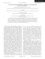
By the way, this was the reflectivity spectrum of a high-temperature superconductor
La1.85Sr0.15CuO4 at 100 K for electric field polarization perpendicular to the CuO2-planes (Ref.
[8]). At this temperature it was not yet superconducting. If you want to fit the reflectivity of the
sample in the superconducting state, I prepared another file for you (“R2.DAT”). Hint: you will
need to introduce an extra Drude term with γ = 0 , which corresponds to the contribution of
superconducting electrons.
3.2. Simultaneous fitting of several data types
This time we consider an example, where several spectra of different types are fitted
simultaneously in order to improve the accuracy of the resulting dielectric function 12 . The
measurements were done on a single-crystalline sample of compound CeIrIn5 at low
temperature T = 35 K (see Ref. [9]). This material is a rather good metal, which results in a
very high reflectivity at low frequencies.
The reflectivity R at nearly-normal incidence was measured in the far- and mid-infrared
spectral range 25 – 5500 cm -1 (data file “R.DAT”). The ellipsometric measurements provided
the spectra of ε 1 and ε 2 from 6000 to 36000 cm -1 , which includes the near-infrared, the visible
and the soft ultraviolet ranges (files “E1.DAT” and “E2.DAT”). In addition, the static (i.e. zerofrequency)
conductivity σ DC , equal to about 4.8 10 4 Ω -1 cm -1 , was obtained from conventional
electrical measurements (file “S1DC.DAT”, which contains only one point).
It is important to fit spectra simultaneously, since it helps to remove the uncertainty,
given by the fact that in the far-infrared only one quantity (reflectivity) is measured, which is in
general not enough to get both ε 1 and ε 2
13 . Therefore, our goal is to fit all available data with
the same model dielectric function. For simplicity, we shall use only the Drude-Lorentz
formula (Equation 2-18).
To begin with, let us load all spectra that we are going to use, one by one. First we load
the reflectivity spectrum.
Please, open the “Dataset Manager” window (Figure 3-6) and click the button in
the first slot. In the window “Load Dataset #1” (shown in Figure 3-7) click the button
on the top. Select the master file “R.DAT” from the directory “TUTORIAL\PART2”. As this
file turns out to be rather big, we will generate a smaller dataset with different set of
frequencies. In the “X” group box check the button “generate” and type 25 in the field “Xmin”,
5000 in the field “Xmax” and 1000 in the field “# pts”. Check the “linear” grid. It means that
the dataset will contain 1000 evenly (linearly) distributed frequency points in the range 25-
5000 cm-1. As a result, the “Load Dataset #1” should look like in Figure 3-20. Click the
button.
12 This example was provided by F.P.Mena
13 One can say, that the knowledge of the static conductivity and as well as high-frequency dielectric function
helps to effectively ‘anchor’ the complex phase of the reflectance coefficient, which is difficult to measure in the
far-infrared
Guide to RefFIT Page 36