software to fit optical spectra - Quantum Materials Group

Guess initial
parameters
p , , p
1 K
START
M
FINISH
YES
Take a small
value of λ
(e.g. λ = 0.
001)
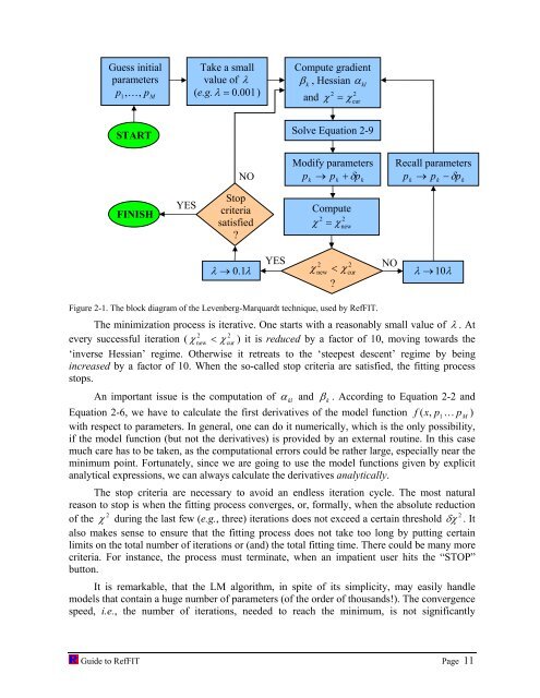
Figure 2-1. The block diagram of the Levenberg-Marquardt technique, used by RefFIT.
NO
Stop
criteria
satisfied
?
λ → 0.
1λ
Compute gradient
β k , Hessian α kl
2 2
and χ = χ
YES 2
χ new
2
< χ cur
?
NO
The minimization process is iterative. One starts with a reasonably small value of λ . At
2 2
every successful iteration ( χ new < χ cur ) it is reduced by a factor of 10, moving towards the
‘inverse Hessian’ regime. Otherwise it retreats to the ‘steepest descent’ regime by being
increased by a factor of 10. When the so-called stop criteria are satisfied, the fitting process
stops.
An important issue is the computation of α kl and β k . According to Equation 2-2 and
Equation 2-6, we have to calculate the first derivatives of the model function f ( x,
p1
K pM
)
with respect to parameters. In general, one can do it numerically, which is the only possibility,
if the model function (but not the derivatives) is provided by an external routine. In this case
much care has to be taken, as the computational errors could be rather large, especially near the
minimum point. Fortunately, since we are going to use the model functions given by explicit
analytical expressions, we can always calculate the derivatives analytically.
The stop criteria are necessary to avoid an endless iteration cycle. The most natural
reason to stop is when the fitting process converges, or, formally, when the absolute reduction
2
2
of the χ during the last few (e.g., three) iterations does not exceed a certain threshold δχ . It
also makes sense to ensure that the fitting process does not take too long by putting certain
limits on the total number of iterations or (and) the total fitting time. There could be many more
criteria. For instance, the process must terminate, when an impatient user hits the “STOP”
button.
It is remarkable, that the LM algorithm, in spite of its simplicity, may easily handle
models that contain a huge number of parameters (of the order of thousands!). The convergence
speed, i.e., the number of iterations, needed to reach the minimum, is not significantly
Guide to RefFIT Page 11
cur
Solve Equation 2-9
Modify parameters
p → p + δp
k
k
Compute
2 2
χ = χ
new
k
Recall parameters
p → p − δp
k
k
λ → 10λ
k