software to fit optical spectra - Quantum Materials Group

extra model type 2, etc. In this case “Einf” is not treated as a parameter but just as model type
identifier and the text labels in the Model window do not have original meanings anymore.
Particular meaning of parameters in the “Lorenzian” section depends on the model type. I must
apologize for such an ‘awkward’ convention, which was temporarily chosen to avoid the major
changes in the program’s user interface. In future RefFIT versions a more elegant way to
distinguish model types will surely be found.
Each model has a set of output quantities, which depends on the model type. Different
quantities are designated by abbreviations. For instance, reflectivity is referred to as “R”, the
real part of conductivity – “S1”, penetration depth – “PD” etc. These abbreviations are
meaningful only for the Dielectric Function model. For other types the meaning of the output
quantities is different, although the same abbreviations are used.
The next sections describe different model types.
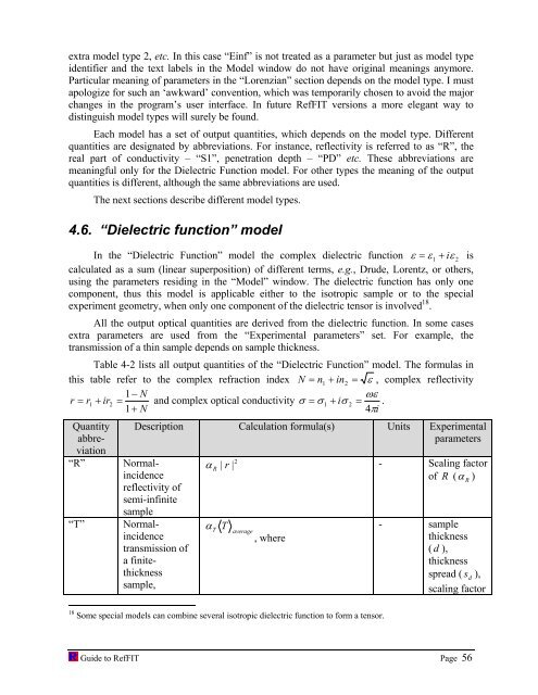
4.6. “Dielectric function” model
In the “Dielectric Function” model the complex dielectric function ε = ε1
+ iε
2 is
calculated as a sum (linear superposition) of different terms, e.g., Drude, Lorentz, or others,
using the parameters residing in the “Model” window. The dielectric function has only one
component, thus this model is applicable either to the isotropic sample or to the special
experiment geometry, when only one component of the dielectric tensor is involved 18 .
All the output optical quantities are derived from the dielectric function. In some cases
extra parameters are used from the “Experimental parameters” set. For example, the
transmission of a thin sample depends on sample thickness.
Table 4-2 lists all output quantities of the “Dielectric Function” model. The formulas in
this table refer to the complex refraction index N = n1
+ in2
= ε , complex reflectivity
1−
N
ωε
r = r1
+ ir2
= and complex optical conductivity σ = σ 1 + iσ
2 = .
1+
N
4πi
Quantity
abbre-
viation
“R” Normalincidence
reflectivity of
semi-infinite
Description Calculation formula(s) Units Experimental
parameters
sample
“T” Normalincidence
transmission of
a finitethickness
sample,
2
α R | r |
- Scaling factor
T T α
average
, where
18 Some special models can combine several isotropic dielectric function to form a tensor.
of R ( α R )
- sample
thickness
( d ),
thickness
spread ( s d ),
scaling factor
Guide to RefFIT Page 56