software to fit optical spectra - Quantum Materials Group

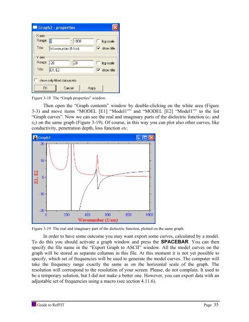
Figure 3-18 The “Graph properties” window.
Then open the “Graph contents” window by double-clicking on the white area (Figure
3-3) and move items “MODEL [E1] “Model1”” and “MODEL [E2] “Model1”” to the list
“Graph curves”. Now we can see the real and imaginary parts of the dielectric function (ε1 and
ε2) on the same graph (Figure 3-19). Of course, in this way you can plot also other curves, like
conductivity, penetration depth, loss function etc.
Figure 3-19 The real and imaginary part of the dielectric function, plotted on the same graph.
In order to have some outcome you may want export some curves, calculated by a model.
To do this you should activate a graph window and press the SPACEBAR. You can then
specify the file name in the “Export Graph to ASCII” window. All the model curves on the
graph will be stored as separate columns in this file. At this moment it is not yet possible to
specify, which set of frequencies will be used to generate the model curves. The computer will
take the frequency range exactly the same as on the horizontal scale of the graph. The
resolution will correspond to the resolution of your screen. Please, do not complain. It used to
be a temporary solution, but I did not make a better one. However, you can export data with an
adjustable set of frequencies using a macro (see section 4.11.6).
Guide to RefFIT Page 35