software to fit optical spectra - Quantum Materials Group

More documents

Recommendations

Info

(Figure 3-8). Using this window one can load up to 10 independent datasets at the same time. One can store more of them, using the macro language (see section 4.11.4). To close the “Dataset Manager” window you can either click the or button. Closing this window helps to save the screen space but does not cause unloading of datasets. 4.8.1. Loading and unloading datasets In order to load a dataset to a certain slot, one should click the button. An extra window will show up, where you can specify the way the data should be loaded to the RefFIT memory. Each dataset is a table, which consists of three columns: X, Y and Yerr. The X is the light frequency (in cm -1 ), the Y is the measured optical quantity (e.g., reflectivity) and the Yerr is the error bar. Figure 4-13 The dataset manager window. One should always specify the master data file. It must contain at least two columns: X and Y. Optionally it may have third column Yerr. The fastest way is to take X, Y and Yerr from the master file. If Yerr is missing, a default value (=0.01) will be put. The data file should be a plain (ANSI) text file. Do not use special text encodings, like UNICODE. The columns in the data file have to be separated by the space character “ “ or the tabulation character. Do not use commas, semicolons etc. Sometimes, it is convenient to have different frequency points in the dataset. For instance, if you load reflection and transmission file, which are measured with different frequency points, you might still want to have two datasets with the same frequency points. In this case there two options. Firstly, you may provide an extra file with only one column – X, which will serve as a source of frequency points. Secondly, you may generate your own grid of frequency points by specifying the interval in the fields “Xmin” and “Xmax”, the number of Guide to RefFIT Page 72
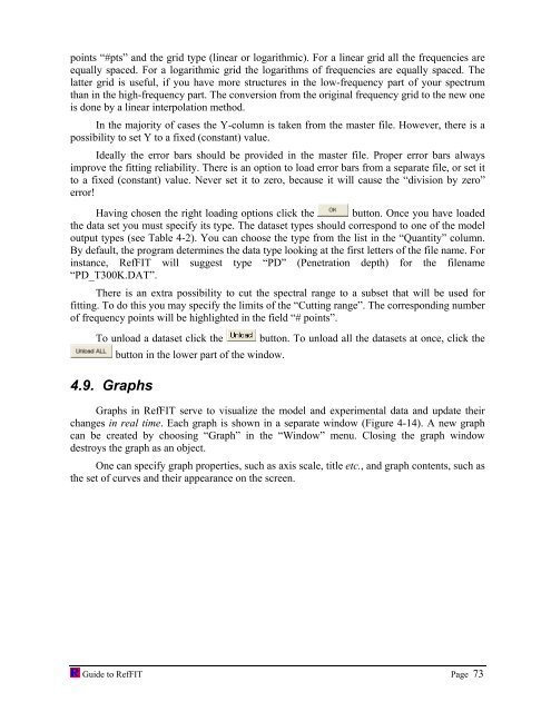
points “#pts” and the grid type (linear or logarithmic). For a linear grid all the frequencies are equally spaced. For a logarithmic grid the logarithms of frequencies are equally spaced. The latter grid is useful, if you have more structures in the low-frequency part of your spectrum than in the high-frequency part. The conversion from the original frequency grid to the new one is done by a linear interpolation method. In the majority of cases the Y-column is taken from the master file. However, there is a possibility to set Y to a fixed (constant) value. Ideally the error bars should be provided in the master file. Proper error bars always improve the fitting reliability. There is an option to load error bars from a separate file, or set it to a fixed (constant) value. Never set it to zero, because it will cause the “division by zero” error! Having chosen the right loading options click the button. Once you have loaded the data set you must specify its type. The dataset types should correspond to one of the model output types (see Table 4-2). You can choose the type from the list in the “Quantity” column. By default, the program determines the data type looking at the first letters of the file name. For instance, RefFIT will suggest type “PD” (Penetration depth) for the filename “PD_T300K.DAT”. There is an extra possibility to cut the spectral range to a subset that will be used for fitting. To do this you may specify the limits of the “Cutting range”. The corresponding number of frequency points will be highlighted in the field “# points”. To unload a dataset click the button. To unload all the datasets at once, click the 4.9. Graphs button in the lower part of the window. Graphs in RefFIT serve to visualize the model and experimental data and update their changes in real time. Each graph is shown in a separate window (Figure 4-14). A new graph can be created by choosing “Graph” in the “Window” menu. Closing the graph window destroys the graph as an object. One can specify graph properties, such as axis scale, title etc., and graph contents, such as the set of curves and their appearance on the screen. Guide to RefFIT Page 73
Page 1 and 2:
Last updated: 20.04.2004 Guide to R
Page 3 and 4:
4.8. Dataset manager ..............
Page 5 and 6:
that time. The later development of
Page 7 and 8:
1.4. Let’s keep in touch Please,
Page 9 and 10:
2.1.1. Levenberg-Marquardt algorith
Page 11 and 12:
Guess initial parameters p , , p 1
Page 13 and 14:
achieve a proper ‘balance’ betw
Page 15 and 16:
The third requirement is that at ve
Page 17 and 18:
Equation 2-19 is useful to estimate
Page 19 and 20:
The first problem is that the Loren
Page 21 and 22: The problem can be circumvented by
Page 23 and 24: In these cases the fitting of the d
Page 25 and 26: 3. Tutorial This chapter shows how
Page 27 and 28: Figure 3-3 Graph contents window is
Page 29 and 30: Figure 3-7 Click the button and in
Page 31 and 32: If you are still far from this fitt
Page 33 and 34: Figure 3-15 The model and experimen
Page 35 and 36: Figure 3-18 The “Graph properties
Page 37 and 38: Figure 3-20 Loading the reflectivit
Page 39 and 40: Figure 3-22 The general RefFIT view
Page 41 and 42: Figure 3-25 The general RefFIT view
Page 43 and 44: MainWindow(XPos = 0, YPos = 0, Widt
Page 45 and 46: emarkable ‘anomaly’, related to
Page 47 and 48: ###################################
Page 49 and 50: # restores the original application
Page 51 and 52: 4. Reference 4.1. System requiremen
Page 53 and 54: Figure 4-2 The “Parameter control
Page 55 and 56: The model file stores information a
Page 57 and 58: considering multiple (Fabri- Perot)
Page 59 and 60: optical conductivity in practical u
Page 61 and 62: Kronig friendly, so be careful! “
Page 63 and 64: function. This command cannot be us
Page 65 and 66: Iinc Itrans ε ε ( 1) ( 2) … (n)
Page 67 and 68: In ellipsometry the complex ratio
Page 69 and 70: ` Figure 4-10 The experimental conf
Page 71: Here ω p and ∞ ε are considered
Page 75 and 76: 4.9.2. Graph contents To set the gr
Page 77 and 78: Available ChiSq terms and click the
Page 79 and 80: At each iteration a linear equation
Page 81 and 82: Before a macro is actually executed
Page 83 and 84: Quantity Text Abbreviation of the q
Page 85 and 86: Parameters: Name Type Description W
Page 87 and 88: “Wp” - plasma frequency; “G
Page 89 and 90: ShowLine Integer =12: Chalk =13: Br
Page 91 and 92: XMin Double Minimal X (frequency) v
Page 93 and 94: always come in pairs. All commands
show all

software to fit optical spectra - Quantum Materials Group

You also want an ePaper? Increase the reach of your titles

Delete template?

Save as template?