software to fit optical spectra - Quantum Materials Group
software to fit optical spectra - Quantum Materials Group
software to fit optical spectra - Quantum Materials Group

Create successful ePaper yourself
Turn your PDF publications into a flip-book with our unique Google optimized e-Paper software.
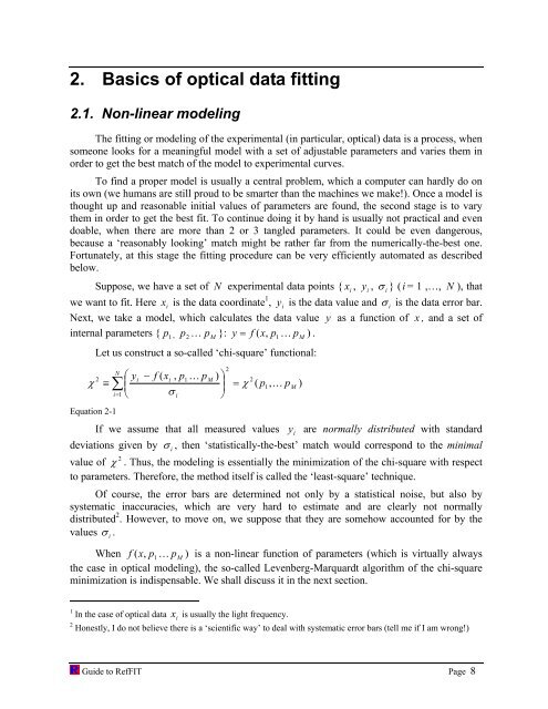
2. Basics of <strong>optical</strong> data <strong>fit</strong>ting<br />
2.1. Non-linear modeling<br />
The <strong>fit</strong>ting or modeling of the experimental (in particular, <strong>optical</strong>) data is a process, when<br />
someone looks for a meaningful model with a set of adjustable parameters and varies them in<br />
order <strong>to</strong> get the best match of the model <strong>to</strong> experimental curves.<br />
To find a proper model is usually a central problem, which a computer can hardly do on<br />
its own (we humans are still proud <strong>to</strong> be smarter than the machines we make!). Once a model is<br />
thought up and reasonable initial values of parameters are found, the second stage is <strong>to</strong> vary<br />
them in order <strong>to</strong> get the best <strong>fit</strong>. To continue doing it by hand is usually not practical and even<br />
doable, when there are more than 2 or 3 tangled parameters. It could be even dangerous,<br />
because a ‘reasonably looking’ match might be rather far from the numerically-the-best one.<br />
Fortunately, at this stage the <strong>fit</strong>ting procedure can be very efficiently au<strong>to</strong>mated as described<br />
below.<br />
Suppose, we have a set of N experimental data points { x i , y i , σ i } (i = 1 ,…, N ), that<br />
we want <strong>to</strong> <strong>fit</strong>. Here x i is the data coordinate 1 , y i is the data value and σ i is the data error bar.<br />
Next, we take a model, which calculates the data value y as a function of x , and a set of<br />
internal parameters { p 1 , 2 p … p M }: y = f ( x,<br />
p1<br />
K pM<br />
) .<br />
Let us construct a so-called ‘chi-square’ functional:<br />
N<br />
2 ⎛ yi<br />
− f ( xi<br />
, p1<br />
K pM<br />
) ⎞ 2<br />
χ ≡ ∑ ⎜<br />
⎟<br />
⎜<br />
= χ ( p1,<br />
K p<br />
i 1 σ ⎟<br />
= ⎝<br />
i ⎠<br />
Equation 2-1<br />
2<br />
If we assume that all measured values y i are normally distributed with standard<br />
deviations given by σ i , then ‘statistically-the-best’ match would correspond <strong>to</strong> the minimal<br />
2<br />
value of χ . Thus, the modeling is essentially the minimization of the chi-square with respect<br />
<strong>to</strong> parameters. Therefore, the method itself is called the ‘least-square’ technique.<br />
Of course, the error bars are determined not only by a statistical noise, but also by<br />
systematic inaccuracies, which are very hard <strong>to</strong> estimate and are clearly not normally<br />
distributed 2 . However, <strong>to</strong> move on, we suppose that they are somehow accounted for by the<br />
values σ i .<br />
When f ( x,<br />
p1<br />
K pM<br />
) is a non-linear function of parameters (which is virtually always<br />
the case in <strong>optical</strong> modeling), the so-called Levenberg-Marquardt algorithm of the chi-square<br />
minimization is indispensable. We shall discuss it in the next section.<br />
1 In the case of <strong>optical</strong> data i<br />
x is usually the light frequency.<br />
2 Honestly, I do not believe there is a ‘scientific way’ <strong>to</strong> deal with systematic error bars (tell me if I am wrong!)<br />
Guide <strong>to</strong> RefFIT Page 8<br />
M<br />
)