software to fit optical spectra - Quantum Materials Group

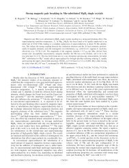
Now we would like to show this curve on the same graph. Let’s go back to the “Graph1”
window and double-click anywhere in the white space. You can notice, that an extra item
“DATA [R] “R1.DAT”” has appeared in the “Available curves” list of the “Graph contents”
window (Figure 3-9). Very nice, this is our dataset. Move it to the “Graph curves” list and click
the button. You may not like the appearance of the experimental curve. If so, you have
to pop up “Graph contents” again, select “DATA [R] “R1.DAT”” in the “Graph curves” list
and set the curve parameters according to your taste. Let us set the parameters as shown in
Figure 3-9.
Figure 3-9 The “graph contents” window with the data and model curves selected for plotting.
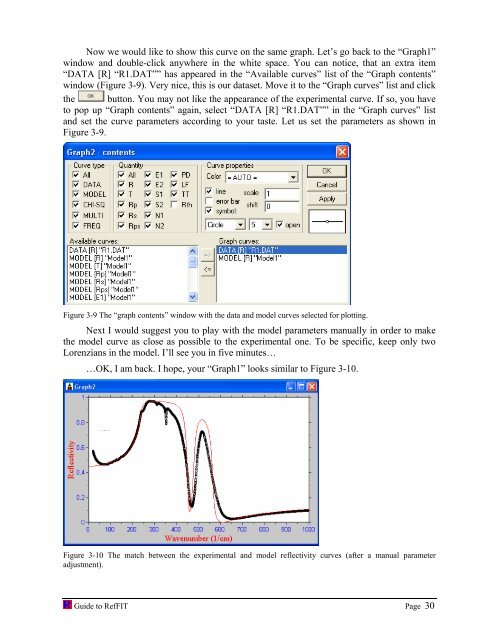
Next I would suggest you to play with the model parameters manually in order to make
the model curve as close as possible to the experimental one. To be specific, keep only two
Lorenzians in the model. I’ll see you in five minutes…
…OK, I am back. I hope, your “Graph1” looks similar to Figure 3-10.
Figure 3-10 The match between the experimental and model reflectivity curves (after a manual parameter
adjustment).
Guide to RefFIT Page 30