software to fit optical spectra - Quantum Materials Group

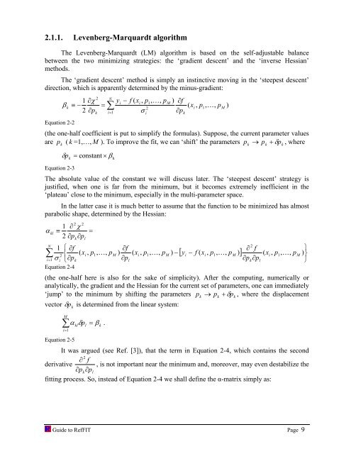
2.1.1. Levenberg-Marquardt algorithm
The Levenberg-Marquardt (LM) algorithm is based on the self-adjustable balance
between the two minimizing strategies: the ‘gradient descent’ and the ‘inverse Hessian’
methods.
The ‘gradient descent’ method is simply an instinctive moving in the ‘steepest descent’
direction, which is apparently determined by the minus-gradient:
β
Equation 2-2
2
1 ∂χ
−
2 ∂p
N
i i 1
k ≡ = ∑ 2
k i= 1 σ i
y
− f ( x , p , K,
p
M
) ∂f
∂p
( x , p , K,
p
(the one-half coefficient is put to simplify the formulas). Suppose, the current parameter values
are p k ( k =1,…, M ). To improve the fit, we can ‘shift’ the parameters pk → pk
+ δpk
, where
δ p = ×
k
Equation 2-3
constant β k
The absolute value of the constant we will discuss later. The ‘steepest descent’ strategy is
justified, when one is far from the minimum, but it becomes extremely inefficient in the
‘plateau’ close to the minimum, especially in the multi-parameter space.
In the latter case it is much better to assume that the function to be minimized has almost
parabolic shape, determined by the Hessian:
2 2
1 ∂ χ
α kl ≡
2 ∂pk
∂pl
=
N 1 ⎧ ∂f
∑ 2 ⎨
i= 1 σ i ⎩∂p
k
Equation 2-4
( xi
, p1,
K,
p
M
∂f
)
∂p
l
( x , p , K,
p
i
1
M
) −
Guide to RefFIT Page 9
k
i
1
M
[ y − f ( x , p , K,
p ) ]
i
i
1
)
M
2
∂ f
∂p
∂p
k
l
( x , p , K,
p
(the one-half here is also for the sake of simplicity). After the computing, numerically or
analytically, the gradient and the Hessian for the current set of parameters, one can immediately
‘jump’ to the minimum by shifting the parameters pk → pk
+ δpk
, where the displacement
vector δ pk
is determined from the linear system:
M
∑
i=
1
Equation 2-5
α δ = β .
kl pl
k
It was argued (see Ref. [3]), that the term in Equation 2-4, which contains the second
∂ f
derivative
∂pk
∂pl
2
, is not important near the minimum and, moreover, may even destabilize the
fitting process. So, instead of Equation 2-4 we shall define the α-matrix simply as:
i
1
M
⎫
) ⎬
⎭