software to fit optical spectra - Quantum Materials Group

function. This command cannot be used before the initialization (button F6).
F5 Toggles between the KK-constrained and non KK-constrained modes. This
command cannot be used before the initialization (button F6).
F6 Initializes the VDF of this model. Attention: the set of the frequency points ω i is
copied from the dataset #1. Make sure, that there is a dataset there! After pressing
F6 the VDF is switched on in the KK-constrained regime and all its parameters
are active in fit (to change that later, use F4, F5 and F7). The initial values of all
parameters are zero.
F7 Toggles the fitting activity of all parameters on and off simultaneously. This
command cannot be used before the initialization (button F6).
Table 4-4 The description of the controls of the variational dielectric function.
The ‘bad news’ is that VDF is not saved together with the model (when using button F2).
However, this shortcoming is easily bypassed by using macros to generate VDFs ‘on-fly’ or by
exporting the model ε 1 and ε 2 to a file.
It worth mentioning that to handle VDF in the KK-constrained mode requires a lot of
computational work and may significantly slow down the program. Therefore one should avoid
the fitting of unnecessary large datasets. On an average modern PC (at the moment of writing
this manual it is Pentium 1.5-2.5 GHz) RefFIT manages easily with N ~ 1000 . Working with
larger datasets would require some patience.
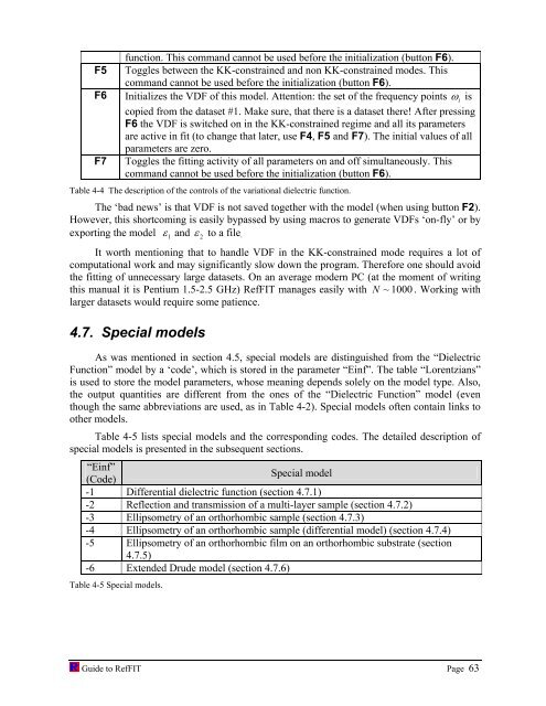
4.7. Special models
As was mentioned in section 4.5, special models are distinguished from the “Dielectric
Function” model by a ‘code’, which is stored in the parameter “Einf”. The table “Lorentzians”
is used to store the model parameters, whose meaning depends solely on the model type. Also,
the output quantities are different from the ones of the “Dielectric Function” model (even
though the same abbreviations are used, as in Table 4-2). Special models often contain links to
other models.
Table 4-5 lists special models and the corresponding codes. The detailed description of
special models is presented in the subsequent sections.
“Einf”
(Code)
Special model
-1 Differential dielectric function (section 4.7.1)
-2 Reflection and transmission of a multi-layer sample (section 4.7.2)
-3 Ellipsometry of an orthorhombic sample (section 4.7.3)
-4 Ellipsometry of an orthorhombic sample (differential model) (section 4.7.4)
-5 Ellipsometry of an orthorhombic film on an orthorhombic substrate (section
4.7.5)
-6 Extended Drude model (section 4.7.6)
Table 4-5 Special models.
Guide to RefFIT Page 63