December 2012 Number 1 - Utah Native Plant Society

Calochortiana December 2012 Number 1
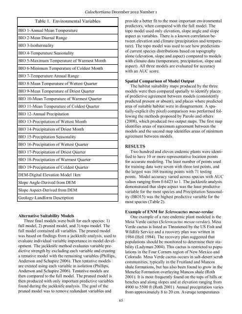
Table 1. Environmental Variables
BIO 1-Annual Mean Temperature
BIO 2-Mean Diurnal Range
BIO 3-Isothermality
BIO 4-Temperature Seasonality
BIO 5-Maximum Temperature of Warmest Month
BIO 6-Minimum Temperature of Coldest Month
BIO 7-Temperature Annual Range
BIO 8-Mean Temperature of Wettest Quarter
BIO 9-Mean Temperature of Driest Quarter
BIO 10-Mean Temperature of Warmest Quarter
BIO 11-Mean Temperature of Coldest Quarter
BIO 12-Annual Precipitation
BIO 13-Precipitation of Wettest Month
BIO 14-Precipitation of Driest Month
BIO 15-Precipitation Seasonality
BIO 16-Precipitation of Wettest Quarter
BIO 17-Precipitation of Driest Quarter
BIO 18-Precipitation of Warmest Quarter
BIO 19-Precipitation of Coldest Quarter
DEM-Digital Elevation Model 1km
Slope Angle-Derived from DEM
Slope Aspect-Derived from DEM
Geology-Landform Description
Alternative Suitability Models
Three final models were built for each species: 1)
full model, 2) pruned model, and 3) topo model. The
full model contained all variables. The pruned model
was based on findings from a jackknife analysis, used to
evaluate individual variable importance in model development.
The jackknife method evaluates variable predictive
strength by excluding each variable and creating
a tentative model with the remaining variables (Phillips,
Anderson and Schapire 2006). Then tentative models
are created using each variable in isolation (Phillips,
Anderson and Schapire 2006). Tentative models are
then compared to the full model. The pruned model is
then produced with only important predictive variables
found during the jackknife analysis. The goal of the
pruned model was to remove redundant variables and
provide a better fit to the most important environmental
predictors, when compared with the full model. The
topo model used only elevation, slope angle and slope
aspect as variables. There is a known correlation between
elevation and climate (precipitation and temperature).
The topo model was used to see how predictions
of current species distributions based on topography
alone (elevation, slope and aspect) compared to models
with climate data (temperature, precipitation, slope and
aspect). All three models are evaluated for accuracy
with an AUC score.
Spatial Comparison of Model Output
The habitat suitability maps produced by the three
models were then compared spatially to identify places
of predictive agreement between models (consistently
predicted present or absent), and places where predicted
area of suitable habitat were in disagreement. A spatially-explicit
(by pixel) comparison was performed following
the methods proposed by Parolo and others
(2008), which produced two output maps. The first map
identifies areas of maximum agreement between the
models and the second map identifies areas of minimum
agreement between models.
RESULTS
Two hundred and eleven endemic plants were identified
to have 10 or more representative location points
for accurate modeling. The least number of points used
for training data were seven with three test points, and
the largest was 168 training points with 71 testing
points. Model accuracy varied across species with AUC
values ranging from 0.6423 to 1. The jackknife analysis
demonstrated that slope aspect was the least predictive
variable for the most species and Precipitation Seasonality
(BIO15) was the highest predictive variable for the
most species (Table 2).
Example of ENM for Sclerocactus mesae-verdae
One example of a rare endemic plant modeled is the
Mesa Verde cactus (Sclerocactus mesae-verdae). Mesa
Verde cactus is listed as Threatened by the US Fish and
Wildlife Service and a recovery plan was written in
1984 (Heil 1984). The recovery plan suggested that
populations should be monitored to determine their stability
(Ladyman 2004). This cactus is restricted to populations
in the Four Corners region of New Mexico and
Colorado. Mesa Verde cactus occurs in salt-desert scrub
communities, typically in the Fruitland and Mancos
shale formations, but has also been found to grow in the
Menefee Formation overlaying Mancos shale (Roth
2001). It is most frequently found on the tops of hills or
benches and along slopes and at elevation ranging from
4900 to 5500 ft (Roth 2001). Annual precipitation varies
from approximately 8 to 20 cm. Average temperatures
65