Annual Meeting - SCEC.org

Report | SCEC Research Accomplishments
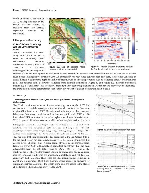
depth of about 70 km (Miller
2011), adding evidence to the
notion that the faulting is
localized from the surface
expression through the
lithosphere.
Lithospheric Scatttering
Role of Seismic Scattering
and the Development of
Coda
Seismic scattering has been
analyzed at CI stations with a
view to examining how
lithospheric structure
contributes to coda (Davis and
Zeng 2011). A full-space
scattering model developed by
Hoshiba (1991) has been applied to coda from stations from the CI network and compared with results from the half-space
layer model developed by Yoshimoto (2000). A comparison has been made between data from Peru, Mexico and California to
assess the role of earthquake depth and lithospheric structure on inferred properties such as scattering, albedo, and mean free
path. The methods seek to separate scattering from intrinsic attenuation (Figure 52 and Figure 53). Intrinsic attenuation
(Figure 53) is significantly less-frequency dependent than scattering attenuation (Figure 52) and may even be frequencyindependent.
Scattering parameters at each station can be used to predict the stochastic part of coda.
Anisotropy
Anisotropy from Mantle Flow Appears Decoupled from Lithospheric
Deformation
The CLM contains estimates of S wave anisotropy to a depth of 635 km
derived from (1) radial anisotropy in the mantle and crust from surface wave
studies (Moschetti et al., 2010) (2) azimuthal anisotropy in the crust and
lithosphere from noise correlation and surface waves (Lin et al., 2011) and (3)
Interpolated SKS estimates in the asthenosphere and lower (Kosarian et al.,
2011). In general SKS directions are parallel to absolute plate motion directions.
Lithospheric azimuthal anisotropy is shown in Figure 54 along withe SKS
splitting. The two disagree in both direction and amplitude with SKS
anisotropy several times larger suggesting splitting originates deeper. The
surface wave anisotropy directions west of the SAF are parallel to the SAF.
This suggests that transpression that has given rise to the San Gabriel Mts in
the big bend region has generated anisotropy in the mantle lithosphere, but
deeper down, absolute plate motion aligns olivines in the asthenosphere.
Figure 55 shows CLM asthenospheric azimuthal anisotropy that has been
extrapolated from the SKS data. Figure 56 (Zandt 2011) is a map of the
southwestern US showing lower crust anisotropy orientations calculated using
receiver functions. Black lines are anisotropy orientations, and red lines are
quaternary fault locations. Blues lines are SKS measurements compiled in
Zandt and Humphreys (2008). Rose diagram shows anisotropy azimuths for
stations in southern California. The length of the lines are related to the plunge
of the fast axis. These data are not yet in the CLM.
76 | Southern California Earthquake Center
Figure 50. Map of sections where
receiver functions are calculated.
Figure 51. Inferred offset of lithosphere beneath
the San Jacinto fault from receiver functions.
Figure 52. Scattering attenuation from coda
Figure 53. Intrinsic attenuation from coda
showing less dependence on frequency
than scattering Q.