Annual Meeting - SCEC.org

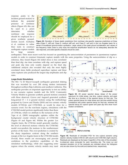
esponse peaks to the
incident ground motion) to
indicate the potential
presence of nonlinear
effects (Figure 63); this can
be used to a priori
determine whether
nonlinear site response
should be employed for a
given synthetic groundmotion
record. Archuleta
et al. continue to refine
their tools to construct
earthquake rupture models
for large scenario
SCEC Research Accomplishments | Report
earthquakes. Their most recent work has focused on quantifying the autocorrelation of parameters in spontaneous rupture
models in order to construct kinematic rupture models with the same properties. Using the autocorrelation of slip as a
reference, they found (Figure 64) initial stress is less correlated
than final slip, rise time correlates with slip, and rupture speed
and peak slip time only weakly depend on the final slip.
Additional analysis also revealed that only the most highly
correlated stress fields produced supershear rupture and these
same ruptures also produced the largest slip amplitudes and slip
rates.
Large-Scale Simulations
The Mw 7.2 El Mayor-Cucapah earthquake generated shaking
that was recorded by over 200 strong motion instruments
throughout northern Baja California and southern California. This
earthquake provides an important opportunity to test our ability
to use scenario rupture models and the SCEC Community
Velocity Models to generate synthetic ground motions consistent
with those observed. Graves and Aagaard generated synthetic
long-period (T > 2 s) ground motions using the methodology
proposed by Graves and Pitarka (2010) and two seismic velocity
models (CVM-4m and CVM-H62), as would be done for a
scenario event. For the non-basin regions, simulations with the
CVM-H62 model perform significantly better than those
of CVM-4m, which we attribute to the inclusion of the
Tape et al. (2009) tomographic updates within the
background crustal velocity structure of CVM-H62
(Figure 65 and Figure 66). Within the greater Los
Angeles basin, the CVM-4m model generally matches
the level of observed motions whereas the CVM-H62
model over-predicts the motions in the southernmost
portion of the basin. This over-prediction is created by
the sharp impedance contrast along the southern
margin of the Los Angeles basin in the CVM-H62 model.
Overall, these results are encouraging and provide
confidence in the predictive capabilities of the
simulation methodology, while also suggesting some
regions where the seismic velocity models may need
Figure 63. Deviation of linear elastic predictions from nonlinear site-specific response predictions at three
sites (Class C: stiff soil, Class D: medium stiff soil, and Class E: soft soil) in the Los Angeles basin for a
series of broadband ground-motion synthetics. Large values of the peak ground acceleration and values of
the frequency index close to unity imply the empirical amplification factors do not adequately describe the
site response, and siste-specific analyses should be used.
Figure 64. 2D power spectral decay (slope of the power
spectrum) for initial stress, rise time, rupture velocity, and peak
slip time as a function of the spectral decay for final slip. The
power spectral decay for initial stress and rise time exhibit strong
correlations with power spectral decay for final slip, whereas the
spectral decay for rupture speed and peak slip time show much
weaker correlations.
Figure 65. Residuals of simulated PGV for one rupture scenario using
seismic velocity models CVM-4m (left column) and CVM-H62 (right column).
Residuals are displayed as the base 2 logarithm of the ratio of the simulatedto-observed
value computed for each recording site. The mean (µ) and
standard deviation (σ) of the residuals are indicated above the histogram
and are also shown by the solid and dashed lines, respectively.
2011 SCEC Annual Meeting | 83