Partielle Differentialgleichungen in der Finanzmathematik Vorlesung ...

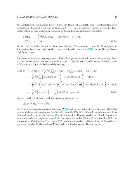
2 DAS BLACK-SCHOLES MODELL 16Zur analytischen Behandlung ist es üblich, die Black-Scholes-DGL zwei Transformationen zuunterziehen. Zunächst wird eine Zeitumkehr t → T − t durchgeführt, dadurch wird das Endwertproblemzu dem analytisch einfacher zu behandelndem Anfangswertproblem∂ t f(t, x) = 1 2 σ2 x 2 ∂ xx f(t, x) + rx∂ x f(t, x) − rf(t, x),f(0, x) = c(x). (2.14)Bei der Interpretation ist nur zu beachten, daß der Zeitparameter t nun die Restlaufzeit derAnlagegüter bezeichnet. Wir werden daher im folgenden auch von (2.14) als der Black-Scholes-Gleichung reden.Als nächstes führen wir die sogenannte Euler-Transformation durch, indem wir y := log x bzw.x = e y substituieren. Sei entsprechend u(t, y) := f(t, e y ) die transformierte Funktion, dannerfüllt u in y = log x die Differentialgleichung∂ t u(t, y) = ∂ t f(t, x) = 1 2 σ2 x 2 d2du(t, log x) + rx u(t, log x) − ru(t, log x)dx2 dx= 1 2 σ2 x 2 d (∂ y u(t, log x) · 1 )+ rx ∂ y u(t, log x) · 1 − ru(t, y)dxxx= 1 ( 12 σ2 x(∂ 2 yu(t, 2 log x) ·x= 1 2 σ2 ∂ 2 yu(t, y) +Entsprechend transformiert sich die Anfangsbedingung zuu(0, y) = f(0, e y ) = c(e y ).) )2+ ∂ y u(t, log x) · −1x 2 + rx ∂ y u(t, log x) · 1 − ru(t, y)x) (r − σ2∂ y u(t, y) − ru(t, y). (2.15)2Der Vorteil der transformierten Gleichung (2.15) liegt darin, daß es sich um eine partielle Differentialgleichungmit konstanten Koeffizienten handelt. Für DGL dieses Typs existieren expliziteLösungsformeln, die wir in Kapitel 4 herleiten werden. Daraus werden wir durch Rücktransformationauch eine explizite Formel für den fairen Preis des Claims C erhalten. Im Falle dereuropäischen Call-Option C = (S T − K) + werden wir so die berühmte Black-Scholes-Formelgewinnen, welche für die moderne Finanzwelt von fundamentaler Bedeutung ist.