Partielle Differentialgleichungen in der Finanzmathematik Vorlesung ...

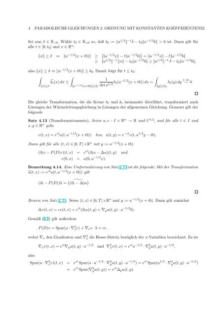
4 PARABOLISCHE GLEICHUNGEN 2. ORDNUNG MIT KONSTANTEN KOEFFIZIENTEN32Sei nun δ ∈ R >0 . Wähle t 0 ∈ R >0 so, daß δ 0 := ‖a 1/2 ‖ −1 δ − t 0 ‖a −1/2 b‖ > 0 ist. Dann gilt füralle t ∈ [0, t 0 ] und x ∈ R n :‖x‖ ≥ δ ⇒ ‖a −1/2 (x + tb)‖ ≥ ∣ ‖a −1/2 x‖ − t‖a −1/2 b‖ ∣ = ‖a −1/2 x‖ − t‖a −1/2 b‖≥ ‖a 1/2 ‖ −1 ‖x‖ − t 0 ‖a −1/2 b‖ ≥ ‖a 1/2 ‖ −1 δ − t 0 ‖a −1/2 b‖,also ‖x‖ ≥ δ ⇒ ‖a −1/2 (x + tb)‖ ≥ δ 0 . Damit folgt für t ≤ t 0 :∫∫∫1˜k t (x) dx ≤‖x‖≥δ‖a −1/2 (x+tb)‖≥δ 0det a 1/2 h t(a −1/2 (x + tb)) dx = h t (y) dy t→0 → 0‖y‖≥δ 0Die gleiche Transformation, die die Kerne h t und k t ineinander überführt, transformiert auchLösungen der Wärmeleitungsgleichung in Lösungen der allgemeinen Gleichung. Genauer gilt derfolgendeSatz 4.13 (Transformationssatz). Seien u, v : I × R n → R und C 1,2 , und für alle t ∈ I undx, y ∈ R n geltev(t, x) = e ct u(t, a −1/2 (x + tb))bzw. u(t, y) = e −ct v(t, a 1/2 y − tb).Dann gilt für alle (t, x) ∈ ]0, T [ ×R n mit y := a −1/2 (x + tb):(∂ t v − P (D)v)(t, x) = e ct (∂ t u − ∆u)(t, y) undv(0, x) = u(0, a −1/2 x).Bemerkung 4.14. Eine Umformulierung von Satz 4.13 ist die folgende: Mit der Transformationũ(t, x) := e ct u(t, a −1/2 (x + tb)) gilt(∂ t − P (D))ũ = ((∂ ˜ t − ∆)u )Beweis von Satz 4.13. Seien (t, x) ∈ ]0, T [ ×R n und y := a −1/2 (x + tb). Dann gilt zunächst∂ t v(t, x) = cv(t, x) + e ct (∂ t u(t, y) + ∇ y u(t, y) · a −1/2 b).Gemäß (4.1) gilt außerdemP (D)v = Spur(a · ∇ 2 xv) + ∇ x v · b + cv,wobei ∇ x den Gradienten und ∇ 2 x die Hesse-Matrix bezüglich der x-Variablen bezeichnet. Es ist∇ x v(t, x) = e ct ∇ y u(t, y) · a −1/2 und ∇ 2 xv(t, x) = e ct a −1/2 · ∇ 2 yu(t, y) · a −1/2 ,alsoSpur(a · ∇ 2 xv)(t, x) = e ct Spur(a · a −1/2 · ∇ 2 yu(t, y) · a −1/2 ) = e ct Spur(a 1/2 · ∇ 2 yu(t, y) · a −1/2 )= e ct Spur(∇ 2 yu(t, y)) = e ct ∆ y u(t, y).