A. Status of the Spectacled Eider - U.S. Fish and Wildlife Service
A. Status of the Spectacled Eider - U.S. Fish and Wildlife Service
A. Status of the Spectacled Eider - U.S. Fish and Wildlife Service

Create successful ePaper yourself
Turn your PDF publications into a flip-book with our unique Google optimized e-Paper software.
As can be seen in Figure 1-2, <strong>the</strong> posterior distributions from <strong>the</strong> three surveys differ quite<br />
dramatically. We used data from <strong>the</strong> last 15 years for all three surveys to estimate a joint<br />
posterior distribution (Figure 1-3). Because <strong>the</strong> surveys were ra<strong>the</strong>r disparate, <strong>the</strong> analysis<br />
required eight million r<strong>and</strong>om selections <strong>of</strong> parameters to obtain <strong>the</strong> posterior distribution.<br />
Although <strong>the</strong> posterior distribution is very broad it is still highly likely that <strong>the</strong> YKD<br />
population has declined over <strong>the</strong> past 15 years.<br />
Figure 1-3. Prior <strong>and</strong> posterior distributions for only <strong>the</strong> last 15 years <strong>of</strong> all three surveys.<br />
The re-sampled 10,000 sets <strong>of</strong> values for <strong>the</strong> eight parameters represents <strong>the</strong>joint posterior<br />
distribution. We utilize this joint posterior distribution to perform a PVA that includes <strong>the</strong><br />
uncertainty in our data (<strong>the</strong> abundance index surveys) <strong>and</strong> <strong>the</strong> model (prior information on<br />
variability in r). We sequentially used each set <strong>of</strong> parameter values as input parameters for a<br />
stochastic population projection. Required input parameters are: N 0, r, <strong>and</strong> s~. Each<br />
simulation began with N0 individuals. The initial number, N0, was drawn from ei<strong>the</strong>r <strong>the</strong> 1995<br />
estimated abundance distribution for <strong>the</strong> Coastal or <strong>the</strong> Ground survey with equal probability.<br />
The simulation proceeded according to equation 1 (below), where r’ was drawn from a Normal<br />
distribution (mean = r, variance = ~ Both <strong>the</strong> time to extinction (