A. Status of the Spectacled Eider - U.S. Fish and Wildlife Service

More documents

Recommendations

Info

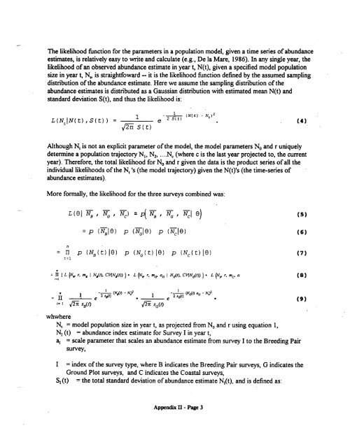
The likelihood function for the parameters in a population model, given a time series ofabundance estimates, is relatively easy to write and calculate (e.g., De la Mare, 1986). In any single year, the likelihood ofan observed abundance estimate in year t, N(t), given a specified model population size in year t, N,, is straightfoward -- it is the likelihood function defined by the assumed sampling distribution of the abundance estimate. Here we assume the sampling distribution ofthe abundance estimates is distributed as a Gaussian distribution with estimated mean N(t) and standard deviation 5(t), and thus the likelihood is: 1 2 1 - ____ (N(t) -Ne) L(N~IN(t),S(t)) = e 2 S(t) (.4) ~‘ThS(t) Although N, is not an explicit parameter ofthe model, the model parameters N 0 and r uniquely determine a population trajectory N1, 2 N~ (where c is the last year projected to, the current year). Therefore, the total likelihood for N0 and r given the data is the product series ofall the individual likelihoods ofthe N, ‘s (the model trajectory) given the N(t)’s (the time-series of abundance estimates). More formally, the likelihood for the three surveys combined was: L(8I NB, N, N) n (5) = p (NBIO) p (NGIO) p (NJ8) (6) n = H p (NB(t) 18) p (NG(t)18) p (N~(t)I8) (7) t=i - II LL(AT.r. m1 N,(r).C~N~(t))). L(NQ. r,m6,a0 I N0Q), CV(N~p))). L(NQ. r, m~.a (B) 2 -~ (NJ:) a~ - N)2 -H I e 2 sit) • e 2sJt) (9) - (NQ) - p~) t- I v’~ s 8(t) vI~i S~3(t) whwhere N, = model population size in year t, as projected from N0 and r using equation 1, N1 (t) = abundance index estimate for Survey I in year t, a1 = scale parameter that scales an abundance estimate from survey Ito the Breeding Pair survey, I index ofthe survey type, where B indicates the Breeding Pair surveys, G indicates the Ground Plot surveys, and C indicates the Coastal surveys, S~ (t) = the total standard deviation of abundance estimate N1(t), and is defined as: Appendix II- Page 3
S 1(t) = m1 CV(N(t)) N(t) (2.0) where = the CV multiplier for survey I, CV(N1(t)) = the estimated survey precision (CV) ofabundance estimate 141(t). Note that parameter values that maximize equation 4 are the maximum likelihood estimates, a common point estimator in frequentist statistics. In Bayesian statistics, rather than maximizing equation 4 we need to integrate the product ofit and the prior distribution ofthe parameters (defined below). Until fairly recently, most Bayesian analyses were restricted to cases where the prior distribution could be chosen so that it was “conjugate” to the likelihood distribution, resulting in their product being a distribution ofa known form, which was integratable by analytic methods. Advances in computing power and numerical and Monte Carlo integration methods have removed this restriction. We use the Sampling-Importance-Resampling routine ofRubin (1988), which Smith and Gelfand (1992) advocate as a particularly useful and simple integration technique for Bayesian statistics. In this method, values for the parameters are randomly selected from their joint prior distribution to form a sample set 0~. The likelihood ofthe data given this particular O~ is calculated and stored. This is repeated, generating n1 O,’s with associated likelihoods. These n1 O,’s are then re-sampled n2 times with replacement, with probability equal to weight q~, where L(011x) (12.) j~1 L(831x) Rubin (1988) showed that this generates a random sample from the joint posterior distribution of size n2. The resampling with replacement from the n1 O,’s with weight CL makes this process analogous to a weighted bootstrap procedure. We set values for n1 and n2 to yield smooth posterior distributions, which depended on the number ofparameters estimated. For single survey analyses, n1 = 300,000, n2 = 5,000. For analyses ofall three surveys, n1 = 8,000,000, n2 = 10,000. For analyses ofall surveys with environmental stochasticity (equation 1), n1 = 25,000,000, n2 = 10,000. With the exception ofinitial population size, prior distributions were Uniform distributions that were iteratively set to encompass the values of the posterior distribution for each parameter. For the full analysis using the deterministic population model (equation 1) and all three data sets, values were randomly drawn from their prior distributions for the seven parameters (r, N0 ma, 1%, a0~ and ar)) to form a 01. Those parameter values were then used to project a model population trajectory using equation 1, forming a series ofmodel population sizes N1, N2, . .N~. The likelihood ofthat population trajectory given the data was then calculated using equation 9, and the 0, ‘s and associated likelihood value were stored. This was repeated n1 times to form the Appendix II- Page 4
Page 2 and 3:
SPECTACLED EIDER RECOVERY PLAN Team
Page 4 and 5:
LITERATURE CITATION U.S. Fish and W
Page 6 and 7:
EXECUTIVE SUMMARY OF THE RECOVERY P
Page 8 and 9:
TABLE OF CONTENTS DISCLAIMER PAGE 1
Page 10 and 11:
LIST OF FIGURES Figure 1. Breeding
Page 12 and 13:
A. Status of the Spectacled Eider R
Page 14 and 15:
) a) j~ 25000 0 2 220000 C ~15000 ~
Page 16 and 17:
B. Causes for Decline and Obstacles
Page 18 and 19:
Increasing interest in avicultural
Page 20 and 21:
Other conservation measures include
Page 22 and 23:
D. Natural History of the Spectacle
Page 24 and 25:
Figure 4. Yukon-Kuskokwim Delta loc
Page 26 and 27:
DEL?A RUSSIA SPECTACLED EIDER RANGE
Page 28 and 29:
helicopter surveys in the Prudhoe B
Page 30 and 31:
geographic populations, because imm
Page 32 and 33:
Figure 8. Study sites and land stat
Page 34 and 35:
their diseases (e.g., Schiller 1954
Page 36 and 37:
E. Distinct Population Segments The
Page 38 and 39:
A final consideration involves info
Page 40 and 41:
Trend data are analyzed to inform w
Page 42 and 43:
Figure 10. A hypothetical posterior
Page 44 and 45:
thresholds are not “magic numbers
Page 46 and 47:
Criteria for Reclassifying from Thr
Page 48 and 49:
Criteria for Delisting from Threate
Page 50 and 51:
The final aspect ofSpectacled Eider
Page 52 and 53:
concordance in their descriptions o
Page 54 and 55:
data on both levels and effects oft
Page 56 and 57:
implicated. In the absence of histo
Page 58 and 59:
. - currently small size of the YKD
Page 60 and 61:
implementation of the Memoranda ofA
Page 62 and 63:
. take of Spectacled Eiders. In add
Page 64 and 65:
. AlS. Produce a handbook summarizi
Page 66 and 67:
. Bl.4. 1.3. Develop visibility cor
Page 68 and 69:
B2. 1.1. Implement YKD satellite tr
Page 70 and 71:
. Appendix Ill). Since epidermal ag
Page 72 and 73:
. feasible if post-fledging staging
Page 74 and 75:
presumed that their activities have
Page 76 and 77:
contaminants within Spectacled Eide
Page 78 and 79:
limited ability to withstand additi
Page 80 and 81:
surface after a year and is no long
Page 82 and 83: . The reproductive stages (eggs, yo
Page 84 and 85: is inadequate to sustain “normal
Page 86 and 87: ___________ 1967. The geese of the
Page 88 and 89: Dementev, G.P., and N.A. Gladkov (e
Page 90 and 91: ___________ 1 964a. Observations on
Page 92 and 93: Nelson, E.W: 1887. Report upon natu
Page 94 and 95: ________ P.R. Wade, R.A. Stehn, and
Page 96 and 97: Robert M. Platte, Migratory Bird Ma
Page 98 and 99: KEY Task Duration and Costs TBD - T
Page 100 and 101: TASK 324.2 I 12.4.1 .2 PRIOR- — 2
Page 102 and 103: TASK I — [37 E12 EI.3 fTYU —PRI
Page 104 and 105: TASK PRIOR- Dj ITYU — — A12.3 2
Page 106 and 107: — TASK U — 135.2 PRIOR- TASK DE
Page 108 and 109: TASK U PRIOR- ITY U TASK DESCRIPTIO
Page 110 and 111: TASK PRIOR. U — DS.3 3 TASK DESCR
Page 112 and 113: The final risk factor is the effect
Page 114 and 115: This PVA will treat two population
Page 116 and 117: Both aerial surveys are conducted a
Page 118 and 119: 0.2 0.15 -j i 4 0.1 0 -I 0.05 0.08
Page 120 and 121: emaining before the population reac
Page 122 and 123: ) critical population size; and (2)
Page 124 and 125: 40%. The population growth rate cri
Page 126 and 127: Table 1-2. Results of simulation wh
Page 128 and 129: Hilborn, R. and C.J. Walters. 1992.
Page 130 and 131: APPENDIX II TECHNICAL DETAILS OF TH
Page 134 and 135: initial sample. Then the O~ were re
Page 136 and 137: LU ~0.8 z -J ~0.6 I-ET1 w107 480 m1
Page 138 and 139: LITERATURE CITED APPENDIX LI De la
Page 140 and 141: where x = age. The fertility rate i
Page 142 and 143: of older females: (1) older females
Page 144 and 145: RESULTS Solutions for single cause
Page 146 and 147: 0.1 0.08 ~0.06 4 0 0.04 0. 0.02 0 0
Page 148 and 149: growth rate. Perhaps this can be mo
Page 150 and 151: decline, by far the fastest way to
Page 152 and 153: LITERATURE CITED APPENDIX In Bailli
Page 154 and 155: APPENDIX IV SPECTACLED EIDER RECOVE
Page 156 and 157: APPENDIX V COMMENTS RECEIVED ON DRA
show all

A. Status of the Spectacled Eider - U.S. Fish and Wildlife Service

Create successful ePaper yourself

Delete template?

Save as template?