The Development of Neural Network Based System Identification ...

86 CHAPTER 4 NEURAL NETWORK BASED SYSTEM IDENTIFICATION
( H
)
∑
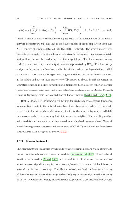
ŷ i (t) = g i W 2 ih V h (t) + B2 i
h=1
+ g i
⎛
⎝
⎞
m∑
W 3 ij X j (t) ⎠ for i = 1, 2, 3 · · · n (4.7)
j=1
where m, n and H denote the number of inputs, outputs and hidden nodes of the HMLP
network respectively, B1 h and B2 i is the bias elements of input and output layer and
X j (t) denotes the inputs data fed into the HMLP network. The weight matrix that
connects the input layer to the hidden layer is given by W 1 hj and W 2 ih indicates weight
matrix that connect the hidden layer to the output layer. The linear connections of
HMLP that connect input and output layer are represented by W 3 ij . The function g h
and g i are the activation function used in the hidden and output layer similar to MLP
architecture. In our work, the hyperbolic tangent and linear activation function are used
in the hidden and output layer respectively. The reason to choose hyperbolic tangent as
activation function in neural network model training is because of its superior learning
speed and accuracy compared with other activation functions such as Bipolar Sigmoid,
Unipolar Sigmoid, Conic Section and Radial Basis Function [Karlik and Olgac, 2010].
Both MLP and HMLP networks can be used for prediction or forecasting time series
by presenting inputs to the network with lags of variables to be predicted. This would
create a set of input variables with delays being fed to the network input layer, which in
turn serve as a short term memory built into network’s weights. This modelling method
using feed-forward network with time lagged inputs is also known as Neural Network
based Autoregressive structure with extra inputs (NNARX) model and its formulation
and representation are given in Section 4.3.2.
4.2.3 Elman Network
The Elman network is a simple dynamically driven recurrent network which attempts to
capture long term history in measurement data [Samarasinghe, 2007]. Elman network
was first introduced by Elman [1990] and it consists of a feed-forward network where
hidden neuron signals are copied to a context/memory units and fed back into the
network in the next time step. The Elman network realised the long term history
of data through its internal memory without relying on externally provided memory
as in NNARX network. Using this recurrence loop concept, the network can develop