The significance of coherent flow structures for the turbulent mixing ...

M
M
^
^
^
g
h
h
þ
Æ
M
Ó
Ó
Ó
*
T
S
c
`
`
M
Æ
M
M
¨
M
6 Investigation of the xz-plane
a particular á9X -position in a plane at Ä can be precisely related to a á9X -position in a plane at
Ä . This is extremely important because any uncontrolled movement of the calibration
ÄZY
target would appear in the correlation data of the velocity fluctuations and could bias the interpretations
of the results, as pointed out in section 3.3. Due to the small spatial separation of
only ten wall-units between the differently polarised light-sheet planes, it was not necessary to
move any camera when changing the measurement position, as all effects could be uniquely
determined by the calibration technique, described in section 3.2, along with the calibration
validation method described in section 3.3. Only the sharpness was slightly adjusted in order
to keep the image contrast and to avoid out-of-focus effects. The determination of the mapping
function was achieved by using the Hough transformation algorithm [18] and the evaluation
of the stereo-scopic images was performed on the DLR SUN-cluster by applying the properly
normalised free-shape correlation described in section 5.2 and [88]. It should be mentioned
that window-deformation techniques, which are increasingly applied for the evaluation of PIV
recordings, are of minor value when the main flow gradients are perpendicular to the lightsheet
plane. This is due to the fact that the variation of the particle image shift inside an interrogation
window is in general not a simple function in contrast to the case where the strong
flow gradients coincide with the measurement plane. For the displacement estimation with
sub-pixel accuracy, a two-dimensional Gaussian peak-fit routine was applied as this approach
is less sensitive to peak-locking effects due to the small variation of the measurement error
with the sub-pixel displacement, see section 2.4.2. By applying the following set of band-pass
and gradient filters ( Æ áJÆ Ó pixel; Î ÄXÆ pixel and M á[HÎ á[
Å]\
pixel), the
number of correct measurements was on average above þ and no smoothing algorithm
T¢T
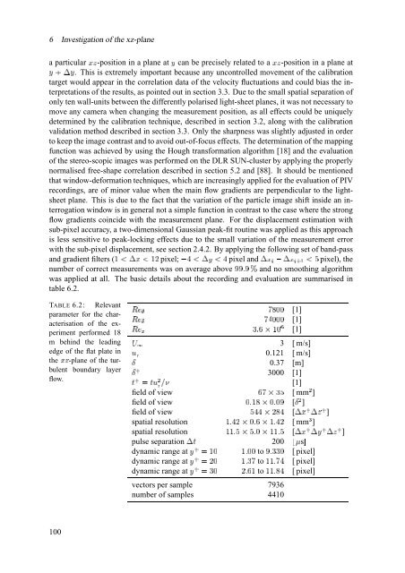
was applied at all. The basic details about the recording and evaluation are summarised in
table 6.2.
TABLE 6.2: Relevant
parameter for the characterisation
of the experiment
performed 18
m behind the leading
edge of the flat plate in
Ú.Q the -plane of the turbulent
boundary layer
flow.
×¥_
×¥a
×b
*:ced
¢
¢ ¢ ¢
`S
þ¡ f
[1]
[1]
[1]
Ô 3 [ m/s]
0.121 [ m/s]
0.37 [m]
3000 [1]
[1]
field of view
field of view
field of view
spatial resolution
spatial resolution
Å W
6 '
þ*:
*“þ
¨k¢ld
.*+ced dj
ed þzþ¢*o¨5dp¨3*+
dj¨
*: dN
[ mm' ]
[Ö ' ] T
[ M á Å ÓS
þ¢*m
þŒþ*o¨
[ M á Å
Ó [ mmn ]
X΁ ]
Ä4Å
X΁ ]
h
pulse separation
dynamic range M W ÄHÅ at
dynamic ÄHÅ W range at
dynamic ÄHÅ W range at
þ¢*: ¢ þ¡
þ¢*:
¢
*:c4þ
to T
to þŒþ¢* ` `
to S
þŒþ¢*
200 qr ss
*:¢¢
[ pixel]
[ pixel]
[ pixel]
vectors per sample 7936
number of samples 4410
100