The significance of coherent flow structures for the turbulent mixing ...
The significance of coherent flow structures for the turbulent mixing ...
The significance of coherent flow structures for the turbulent mixing ...

You also want an ePaper? Increase the reach of your titles
YUMPU automatically turns print PDFs into web optimized ePapers that Google loves.
¾<br />
–<br />
’<br />
–<br />
5 Investigation <strong>of</strong> <strong>the</strong> xy-plane<br />
<strong>the</strong> log-law holds, is quite large <strong>for</strong> both cases so that a direct interaction between <strong>the</strong> nearwall<br />
<strong>flow</strong> structure with <strong>the</strong> intermittent <strong>flow</strong> region can not take place. Thus <strong>the</strong> <strong>turbulent</strong><br />
<strong>flow</strong> state can be considered as fully developed. Fully developed <strong>flow</strong>s are characterised by<br />
a Kolmogorov cascade including an inertial range over at least one order <strong>of</strong> magnitude in <strong>the</strong><br />
wavenumber space [78]. This condition implies unsteadiness, rotational, three-dimensionality,<br />
non-deterministic, diffusion and dissipation, e.g. attributes which are generally referred to<br />
characterise <strong>turbulent</strong> <strong>flow</strong>s. <strong>The</strong> dynamic <strong>of</strong> <strong>the</strong> velocity signal as a function <strong>of</strong> <strong>the</strong> wall distance<br />
can be estimated from figure 5.3 which shows <strong>the</strong> normalised rms values <strong>of</strong> <strong>the</strong> three<br />
velocity fluctuations <strong>for</strong> both <strong>flow</strong> cases. It can be seen that <strong>the</strong> maximum can be properly<br />
resolved with state-<strong>of</strong>-<strong>the</strong>-art PIV systems, provided <strong>the</strong> magnification <strong>of</strong> <strong>the</strong> imaging system<br />
is well adjusted relative to <strong>the</strong> <strong>flow</strong> <strong>structures</strong> and <strong>the</strong> problems associated with <strong>the</strong> strong wall<br />
reflections are solved. <strong>The</strong> low Reynolds number results agree quite well with <strong>the</strong> HWA measurements<br />
kindly provided by Pr<strong>of</strong>. Dr. Fernholz. Only <strong>the</strong> first two measurement points near<br />
<strong>the</strong> wall are overestimated. This is natural due to <strong>the</strong> finite size <strong>of</strong> <strong>the</strong> measurement volume.<br />
When <strong>the</strong> high Reynolds number results are considered <strong>the</strong> deviation increases but <strong>the</strong> increase<br />
<strong>of</strong> <strong>the</strong> second peak with increasing Reynolds number is clearly visible and in agreement with<br />
<strong>the</strong> literature [21]. To validate <strong>the</strong> degree <strong>of</strong> anisotropy between different velocity components<br />
in <strong>turbulent</strong> shear <strong>flow</strong>s, <strong>the</strong> ratio between orthogonal velocity fluctuations is shown in<br />
<strong>the</strong> right graphs <strong>of</strong> <strong>the</strong> same figure. As <strong>the</strong> energy from <strong>the</strong> mean motion is first transferred into<br />
<strong>the</strong> stream-wise velocity fluctuation be<strong>for</strong>e <strong>the</strong> transfer into ³ <strong>the</strong> ´ and component takes place<br />
by means <strong>of</strong> pressure fluctuations, <strong>the</strong> value <strong>of</strong> <strong>the</strong> anisotropy parameter is usually around 0.6<br />
<strong>for</strong> large wall distances. In addition, it can be seen µ ³ ¬' ·E¬'¸ ±º¹ ¬ that increases gradually with<br />
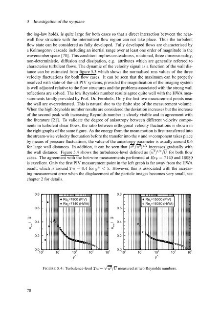
<strong>the</strong> wall distance. Figure 5.4 shows <strong>the</strong> turbulence-level defined µ · ¬ ¸ ±º¹ ¬ » as <strong>for</strong> both<br />
~½¿¾7À<br />
<strong>flow</strong><br />
’¥ÁŒŒÂŒ and<br />
cases. <strong>The</strong> agreement with <strong>the</strong> hot-wire measurements per<strong>for</strong>med ¼ at<br />
is excellent. Only <strong>the</strong> first PIV measurement point in <strong>the</strong> left graph is far away from <strong>the</strong> HWA<br />
result, which is à · 4‘<br />
around Ä4Å