The significance of coherent flow structures for the turbulent mixing ...

æ
æ
æ
æ
æ
æ
ã
ã
ã
H
H
H
I
I
I
I
I
I
I
ã
ã
ã
6 Investigation of the xz-plane
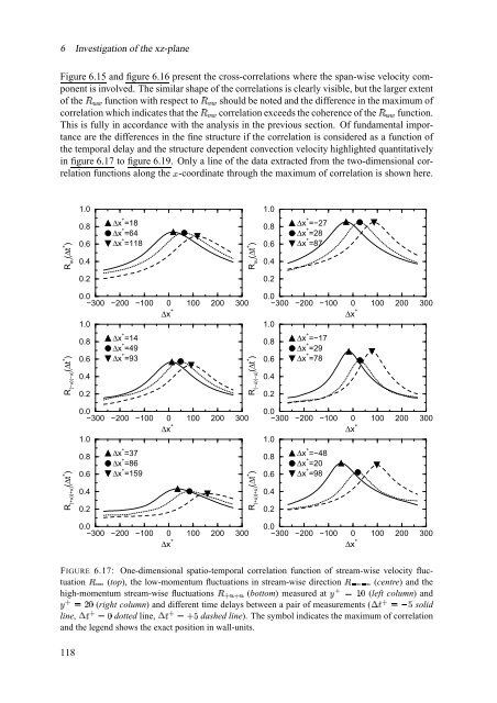
Figure 6.15 and figure 6.16 present the cross-correlations where the span-wise velocity component
is involved. The similar shape of the correlations is clearly visible, but the larger extent
of the Ã Ñ function with respect to ÃË should be noted and the difference in the maximum of
correlation which indicates that the ÃË correlation exceeds the coherence of the à Ñ$ function.
This is fully in accordance with the analysis in the previous section. Of fundamental importance
are the differences in the fine structure if the correlation is considered as a function of
the temporal delay and the structure dependent convection velocity highlighted quantitatively
in figure 6.17 to figure 6.19. Only a line of the data extracted from the two-dimensional correlation
functions along the Î -coordinate through the maximum of correlation is shown here.
1.0
1.0
R uu
(∆t + )
0.8
0.6
0.4
æ
∆x + =18
∆x + =64
∆x + =118
t + )
R uu
(∆
0.8
0.6
0.4
I
∆x + =−27
∆x + =28
∆x + =87
0.2
0.2
ã
0.0
−300 −200 −100 0 100
∆x
1.0
200
ã
300
ã
0.0
−300 −200 −100
1.0
ã
0
∆x
+
100
ã
200
ã
300
ã
R (−u)(−u)
(∆t + )
0.8
0.6
0.4
0.2
æ
∆x + =14
∆x + =49
∆x + =93
t + )
R (−u)(−u)
(∆
0.8
0.6
0.4
0.2
∆x + =−17
∆x + =29
∆x + =78
ã 0.0
−300 −200 −100 0 100
∆x +
1.0
200
ã
300
ã
0.0
−300 −200 −100
1.0
ã
0
∆x +
100
ã
200
ã
300
ã
R (+u)(+u)
(∆t + )
0.8
0.6
0.4
0.2
æ
∆x + =37
∆x + =86
∆x + =159
t + )
R (+u)(+u)
(∆
0.8
0.6
0.4
0.2
I
∆x + =−48
∆x + =20
∆x + =98
ã
0.0
−300 −200 −100 0 100
∆x
200
ã
300
ã
0.0
−300 −200 −100
ã
0
∆x
+
100
ã
200
ã
300
ã
FIGURE 6.17: One-dimensional spatio-temporal correlation function of stream-wise velocity fluctuation
(top), the low-momentum fluctuations in stream-wise Ð î Ñ î Ñ direction (centre) and the
ÐÒјÑ
high-momentum stream-wise Ð ® Ñ ® Ñ fluctuations (bottom) measured Ó ® Ü Ø
at (left column) and
® Ú¥Ø
(right column) and different time delays between a pair of measurements (KJ ® ú ù
solid
Ó
J ® Ø
line, dotted KJ ® L6 ù
line, dashed line). The symbol indicates the maximum of correlation
and the legend shows the exact position in wall-units.
118