The significance of coherent flow structures for the turbulent mixing ...
The significance of coherent flow structures for the turbulent mixing ...
The significance of coherent flow structures for the turbulent mixing ...

Create successful ePaper yourself
Turn your PDF publications into a flip-book with our unique Google optimized e-Paper software.
%<br />
{<br />
s<br />
s<br />
s<br />
s<br />
7.1 Experimental set-up<br />
For <strong>the</strong> evaluation <strong>of</strong> <strong>the</strong> stereo-scopic images <strong>the</strong> second order warping technique was<br />
applied again, along with <strong>the</strong> calibration validation procedure described in section 3.3. This<br />
ensures that <strong>the</strong> interrogation spots from each <strong>of</strong> a pair <strong>of</strong> stereo-scopic images correspond<br />
to <strong>the</strong> same region <strong>of</strong> <strong>the</strong> <strong>flow</strong>. <strong>The</strong> interrogation <strong>of</strong> <strong>the</strong> data was per<strong>for</strong>med with <strong>the</strong> FFTbased<br />
free shape cross-correlation outlined in section 2.4, and <strong>for</strong> <strong>the</strong> determination <strong>of</strong> <strong>the</strong><br />
signal-peak with sub-pixel accuracy, <strong>the</strong> two-dimensional Gaussian fit using <strong>the</strong> Levenberg-<br />
Marquardt method has been applied. This peak finding method is less sensitive to sub-pixel<br />
displacements compared with <strong>the</strong> three point Gaussian peak fit, see figure 2.14 and table 2.1 <strong>for</strong><br />
h ¨ji h ¨<br />
À ¤lknm hpo¥ÍeÏpo À k<br />
oüÍrq8o Ç Í5Î Í5ÎEs > out Ç<br />
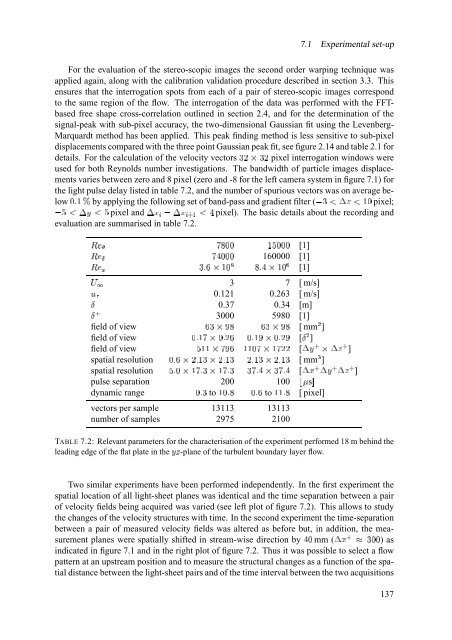
details. For <strong>the</strong> calculation <strong>of</strong> <strong>the</strong> velocity vectors pixel interrogation windows were<br />
used <strong>for</strong> both Reynolds number investigations. <strong>The</strong> bandwidth <strong>of</strong> particle images displacements<br />
varies between zero and 8 pixel (zero and -8 <strong>for</strong> <strong>the</strong> left camera system in figure 7.1) <strong>for</strong><br />
<strong>the</strong> light pulse delay listed in table 7.2, and <strong>the</strong> number <strong>of</strong> spurious vectors was on average below<br />
by applying <strong>the</strong> following set <strong>of</strong> band-pass and gradient filter ( pixel;<br />
pixel and pixel). <strong>The</strong> basic details about <strong>the</strong> recording and<br />
evaluation are summarised in table 7.2.<br />
[1]<br />
160000 [1]<br />
[1]<br />
0.37 0.34 [m]<br />
3000 5980 [1]<br />
ÿ 3 7 [ m/s]<br />
| ¡ 0.121 0.263 [ m/s]<br />
s %<br />
field <strong>of</strong><br />
Þ h ijÆ É Þ h iNÆ É view mmá [ ]<br />
field <strong>of</strong> À ¤}k È i À ¤ ¨ Þ À ¤lk Æji À ¤ ¨$Æ<br />
view [ á ]<br />
field <strong>of</strong> view % kk i È Æ Þ kk ÀÈ i k È ¨¨ [Írq<br />
s i ÍlÏ<br />
Ç<br />
spatial À ¤:Þ i~¨ ¤}k h i~¨ ¤}k h ¨ ¤lk h i ¨ ¤lk h resolution [ mm ]<br />
spatial resolution B ¤ À i k È ¤ h i k È ¤ h hÈ ¤ t i hÈ ¤ t [Í5Î<br />
Ç<br />
]<br />
]<br />
€ s‚<br />
À h ¤ k ¤ É À ¤:Þ À kk¤ É<br />
pulse separation 200 100<br />
dynamic range to to [ pixel]<br />
vectors per sample 13113 13113<br />
number <strong>of</strong> samples 2975 2100<br />
Írq<br />
ÍeÏ<br />
TABLE 7.2: Relevant parameters <strong>for</strong> <strong>the</strong> characterisation <strong>of</strong> <strong>the</strong> experiment per<strong>for</strong>med 18 m behind <strong>the</strong><br />
leading edge <strong>of</strong> <strong>the</strong> flat plate in <strong>the</strong> Óc -plane <strong>of</strong> <strong>the</strong> <strong>turbulent</strong> boundary layer <strong>flow</strong>.<br />
Two similar experiments have been per<strong>for</strong>med independently. In <strong>the</strong> first experiment <strong>the</strong><br />
spatial location <strong>of</strong> all light-sheet planes was identical and <strong>the</strong> time separation between a pair<br />
<strong>of</strong> velocity fields being acquired was varied (see left plot <strong>of</strong> figure 7.2). This allows to study<br />
<strong>the</strong> changes <strong>of</strong> <strong>the</strong> velocity <strong>structures</strong> with time. In <strong>the</strong> second experiment <strong>the</strong> time-separation<br />
between a pair <strong>of</strong> measured velocity fields was altered as be<strong>for</strong>e but, in addition, <strong>the</strong> measurement<br />
planes were spatially shifted in stream-wise direction by tÀ mm (Í5Î<br />
indicated in figure 7.1 and in <strong>the</strong> right plot <strong>of</strong> figure 7.2. Thus it was possible to select a <strong>flow</strong><br />
pattern at an upstream position and to measure <strong>the</strong> structural changes as a function <strong>of</strong> <strong>the</strong> spatial<br />
distance between <strong>the</strong> light-sheet pairs and <strong>of</strong> <strong>the</strong> time interval between <strong>the</strong> two acquisitions<br />
s Ê h¢À¢À ) as<br />
137