The significance of coherent flow structures for the turbulent mixing ...
The significance of coherent flow structures for the turbulent mixing ...
The significance of coherent flow structures for the turbulent mixing ...

Create successful ePaper yourself
Turn your PDF publications into a flip-book with our unique Google optimized e-Paper software.
!<br />
6 Investigation <strong>of</strong> <strong>the</strong> xz-plane<br />
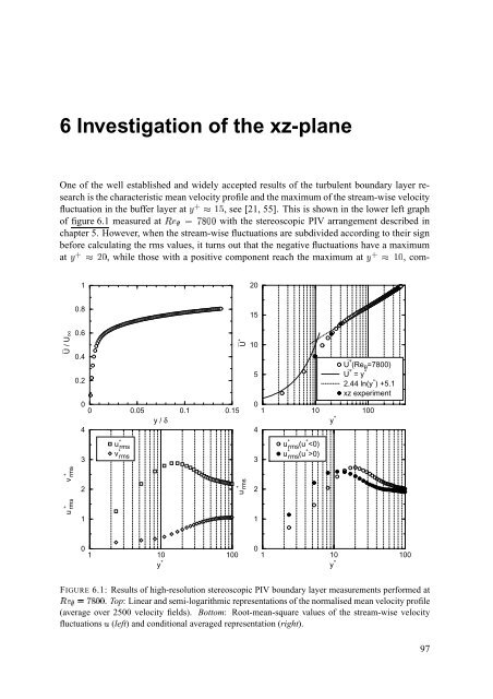
One <strong>of</strong> <strong>the</strong> well established and widely accepted results <strong>of</strong> <strong>the</strong> <strong>turbulent</strong> boundary layer research<br />
is <strong>the</strong> characteristic mean velocity pr<strong>of</strong>ile and <strong>the</strong> maximum <strong>of</strong> <strong>the</strong> stream-wise velocity<br />
fluctuation in <strong>the</strong> buffer layer at ¢¡¤£¦¥¨§ , see [21, 55]. This is shown in <strong>the</strong> lower left graph<br />
<strong>of</strong> figure 6.1 measured at © with <strong>the</strong> stereoscopic PIV arrangement described in<br />
chapter 5. However, when <strong>the</strong> stream-wise fluctuations are subdivided according to <strong>the</strong>ir sign<br />
be<strong>for</strong>e calculating <strong>the</strong> rms values, it turns out that <strong>the</strong> negative fluctuations have a maximum<br />
at ¡£ , while those with a positive component reach <strong>the</strong> maximum at ¡£¥ , com-<br />
1<br />
20<br />
0.8<br />
15<br />
∞<br />
⎺U / U<br />
0.6<br />
0.4<br />
0.2<br />
0<br />
0<br />
0.05 0.1 0.15<br />
y /<br />
δ<br />
4<br />
3<br />
u + rms<br />
v + rms<br />
+<br />
⎺U<br />
10<br />
5<br />
0<br />
4<br />
3<br />
10 100 <br />
1<br />
y +<br />
u + rms (u+ 0)<br />
⎺U + (Re θ =7800)<br />
⎺U + = y +<br />
2.44 ln(y + ) +5.1<br />
xz experiment<br />
+<br />
+<br />
u +<br />
rms v +<br />
rms<br />
2<br />
1<br />
u +<br />
rms<br />
2<br />
1<br />
0<br />
y +<br />
10 100<br />
1<br />
0<br />
1 <br />
10 100<br />
y +<br />
FIGURE 6.1: Results <strong>of</strong> high-resolution stereoscopic PIV boundary layer measurements per<strong>for</strong>med<br />
"$#<br />
at<br />
. Top: Linear and semi-logarithmic representations <strong>of</strong> <strong>the</strong> normalised mean velocity pr<strong>of</strong>ile<br />
&%(')*+*<br />
(average over 2500 velocity fields). Bottom: Root-mean-square values <strong>of</strong> <strong>the</strong> stream-wise velocity<br />
, fluctuations (left) and conditional averaged representation (right).<br />
97